Snow Solver in PreonLab

September 30, 2021
Fabian Meyer and Marian Majda

Snow creates deeply physical experiences that can remain vivid memories: Seeing snow for the first time, a snow crystal melting on your tongue, a snowball fight, the different activities summarized as winter sports. However, snow also affects human activity and can, quite literally, get in the way. Snowplows clear roads, highways, airfields and railroads. Snow drifts may destabilize structures due to uneven loading. Avalanches and blizzards are natural hazards that can endanger living beings.

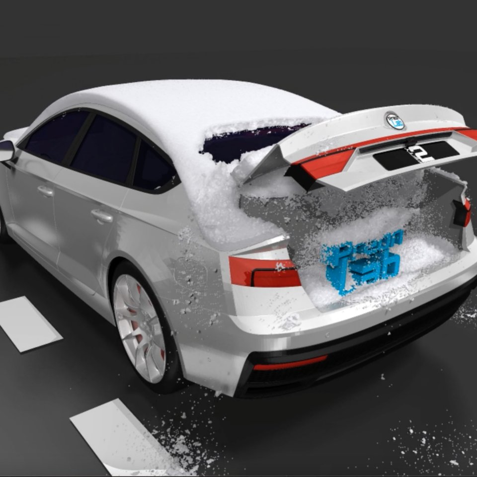
PreonLab solves many automotive problems. When it comes to snow, one is foremost interested to prevent soiling of critical components. The number of tasks is vast. Some that PreonLab has already solved are: Placing cameras for self-driving cars, snow entering the engine air intake which can cause a power drop or localizing corrosion hot-spots in the wheelhouse. Audi and Great Wall Motor are just some examples demonstrating the snow solver capabilities to simulate and capture phenomenas measured in real world test setups at different vehicle speeds. Out of the many sensors PreonLab provides, the addition of the height sensor has been key for the engineers to assess soiling.

So how does PreonLab achieve this? Let’s take a step back and look what we are up against.

Share:

The Challenge

Liquids only noticably compress under extraordinary high pressures and are thus often assumed to be incompressible. The bulk modulus of water is 2,2⋅109 Pa and thus offers high resistance to density changes. Quite contrary, the bulk modulus of snow is of order 1⋅105 Pa. Thus compression is much easier achieved in pressure ranges we are accustomed to.

Most liquid effects are immediate and don’t require knowledge of the history of the fluid. As discussed above density changes are almost immediately resolved. Analogous, viscosity also only requires a notion of surrounding velocities to determine the shear stress. In particular no knowledge of previous states of the fluid.

Snow is different in this regard. An elasto-plastic model has been proven to be quite powerful to model snow. The resisting stress is dependent on the initial unloaded state. So, exactly one point in history. The larger the deformation from that state the larger the resulting stress will be. As long as the deformation is small the snow will recover its original appearance. This effect is called elasticity and is the result of the bonds in the crystalline structure of solids that will rearrange to the original appearance when external pressure is released. As discussed above, the bonds are comparatively weak to other materials which brings us to the next effect: plasticity. If the bonds change, the damage done is unrecoverable and the appearence of the snow will change lastingly.

Snow in contrary to fluids has quite a large variety of dynamics. These are dependent on other historic factors the snow has undergone. Chunky snow can be found when it was exposed to temperatures around the freezing point. If its colder, snow tends to be more powdery. The content of water/ice is also crucial but we will face that later.

Please agree to the transfer of data to third parties as set out in our privacy policy.

Height Sensor in PreonLab

The Solution

Stomakhin et al. [2013] pioneered the elasto-plastic treatment of snow for computer graphics for its animation film “Frozen”. The model has since then been adapted for avalanche research in Gaume et al. [2018] proving its power. The adaption to SPH and further modeling we do in PreonLab is described by Gissler et al. [2020]. Many of the authors of this paper are working and researching at FIFTY2 Technology GmbH: Christoph Gissler, Andreas Henne and Andreas Peer. Since the publication of the article last year, we have been refining the methods further.

PreonLab does not have any microscopic modeling of tracking bonds, nor does it store the unloaded state. It stores a measure of the current elastic and plastic deformation accumulated over time. In 3D, per SPH interpolation point, we need to store the elastic deformation, a 3×3 matrix, and the plastic deformation which is a scalar. Furthermore, a 3×3 matrix for the stress is needed. The snow solver thus requires comparably more memory than a Preon Solver (about 2.5x for the same number of particles).

The Cauchy momentum equation describes how the Snow Solver moves forward in time. The Cauchy Stress tensor σ creates the elasto-plastic forces of the snow and ƒ are other body forces, e.g., gravity or wind. We assume hyperelasticity, thus the stress tensor comes from an elasto-plastic energy density function whose inputs are the elastic​ FE and plastic FP deformation gradients. Multiplicative plasticity theory divides up deformation into elastic recoverable and plastic permanent parts F=FEFP.

For small strains the corotated linear elasticity model is sufficient. We allow the singular values of FE to be between [1−θc, 1+θs] which corresponds to restricting principal strains. All excess is attributed to FP. We thus don’t explicity model a stress yield surface and flow rule like Gaume et al. [2018].

Strain hardening is realized by modifying the Lamé parameters , with an exponential function. As input it takes the plastic deformation Jp= det(Fp) which is scaled by the hardening parameter ξ. In addition, we modify Jp to incorporate a notion of density to allow for accumulation of snow. E controls the overall strength of the stress response, μ the amount of shearing.

We discretize the Cauchy momentum equation in time with Backward Euler. We do two seperate discretizations of spatial derivatives using SPH: The gradient of velocity to get the strain rate ϵt+Δt and the divergence of stress which we encountered in the Cauchy momentum equation. The Lamé parameters are kept constant to get a linear system we can solve for. We use BiCGSTAB since the system is not guaranteed to be symmetric.

That was quite a lot to take in. How can you use it?

Please agree to the transfer of data to third parties as set out in our privacy policy.

Snow in Trunk in PreonLab

Snow Types

We elaborated that historic effects influence the snow type. Exposure to different temperatures, melting and refreezing, saturation have a significant effect on the type.

Although a coupling with temperature, simulating phase changes and tracking water/ice content would be nice, the range of parameters becomes increasingly large; For us and the customer to evaluate. For a stand-alone model its much more efficient to parametrize the effective range of dynamics of snow. For now that’s what we do and still allows coupling in the future.

Since we supply six parameters ρ, E, ν, θc, θs, ξ to modify the snow behavior to your needs, the practical range is still enormous. PreonLab thus introduced with version 4.3 snow types which are good starting points to cater to the effects you observe. These 6 types are:

  • default, a good starting point for the first simulation
  • powdery, for modelling very brittle snow splitting into many snow particles
  • chunky, for modelling sticky snow splitting into clusters of snow particles
  • icy, for snow that offers much resistance to external forces
  • watery, for modelling snow that has high water content and its appearence goes into the viscous fluid range
  • muddy (or slush) as a mixture of water and snow that shows splashing and bow-wave behavior

We observed that most of the time our customers are satisfied with choosing one of the snow types and not modifying them further. However the presets directly map onto five of the underlying parameters which you can easily inspect in the Property Editor of PreonLab. So you can tweak them as you like to combine the effects. For a more detailed description about the parameters you should refer to the manual. The one parameter not modified is the density which leaved the closed-off snow-system and also modifies external forces, like air flows.

Please agree to the transfer of data to third parties as set out in our privacy policy.

Snow Defaults in PreonLab

It's PreonLab!

The snow solver is one of the solvers that are included in PreonLab. This means that you get all the other advantages of PreonLab as well!

One of PreonLab’s core advantages is the low effort needed for preprocessing. A good example for this ease of use is the setting up of geometries of boundaries which often can be done in a few minutes. Interactions between objects in Preonlab can be arranged intuitively in the Connection Editor. Postprocessing like evaluating sensors and highly realstic rendering via the Preon renderer is fully integrated with PreonLab and easy to use.

The Lagrangian treatment of constitutive equations easily solves convection. The implicit solver increases the stability of the simulation and allows the user to run simulations with large time steps. Additionally PreonLab features MPI for computations on several nodes which can speed up the computations and makes it possible to scale to more challenging simulation scenarios.

Next up!

We have been constantly improving the quality of the snow solver. For PreonLab 5.0 we improved visual snow quality by starting the solver with an educated, physical guess for the final velocity. This takes some computational effort, but lowers the number of needed iterations per time step for the same quality.

The upcoming release PreonLab 5.1 this fall, will feature a snow solver that will be faster than ever before. PreonLab 5.1 will include a preconditioning of the linear system matrix to reduce iterations even further. More news about these two interesting innovations will be shown in an upcoming article, so stay tuned.

Update: the new article is now online and ready for you to read! Find it here.

RELATED ARTICLES

LEARN MORE ABOUT PreonLab Updates

How to get started with
Preonlab CFD software?
Get in Touch