An Optimized Snow Solver

To solve a time-dependent partial different equation like the Cauchy Momentum equation for the snow solver we use an implicit method. Specifically, the Backward Euler method. Implicit methods not only rely on the current (particle) state but also on the future one. This state is, by definition, unknown. The magic of implicit methods is to treat this unknown future information as a variable like the others and work from that. This results in a system of linear equations. It is extra effort but it leads to more stable equations and allows to use a significantly higher timestep.

We write the system of equations as Av^t+Δt=v^*, where the following notation is used.

For snow the unknowns are the future velocities v^t+Δt. The known velocities v^* also consist of explicitly applied accelerations like gravity or air and the predicted elastic accelerations (that we are going to correct). The components of the matrix A consist of the smoothed particle hydrodynamics (SPH) space discretizations of the partial differential equation. Thus each snow particle leads to additional rows in the system of equations. More precisely, we get an unknown for each dimension in space per particle. Usually, this means 3 unknown variables per particle. This typically results in a very large linear system. Using Gaussian elimination or other direct methods is very time (and memory) consuming.

Iterative methods make for a very efficient alternative. These methods try with each step (or iteration) to get closer to the solution of that partial differential equation, see above image. If the solution is sufficiently close to solving the equation, i.e. if a user defined error is reached, we accept that solution. The error thus gives a very good controlling mechanism on how accurate the system should be solved for. Thus, higher accuracy implies more iterations and consequently more computation time.

Enough with all the math talk, let’s look at a particular scene in PreonLab 4.3.3:

The higher accuracy in the right image results in chunkier snow on the ground while on the left the snow is very brittle, almost like sand. However, the higher accuracy has its costs. Here are the iteration statistics of the snow solver in the wedge scene:

The average iteration numbers are much higher due to the required lower error margin. Also over time the number of iterations are quite erratic and suddenly jump up and down. On the left we have six and on the right ten jump ups. So what happens at these jumps? Following above, at a jump up the solver suddenly encounters a problem that’s very hard. The first jump down is actually natural and the solver recovered on its own. On all other jump downs however the problem was not only very hard to solve but sadly reached a state where we did not get closer to the solution at all.

PreonLab 4.2.0 therefore introduced a rescue mechanism (fall back) to do an explicit step instead. This rescue mechanism saved simulations from explosions and very heavy particle deletion but still deleted a considerable amount of particles. Problematic particles leading to the jump up were likely to be deleted by this rescue step. As a consequence iterations would immediately jump down again. We knew this wasn’t satisfactory and only an intermediate solution.

The first challenge is to reduce the amount of jumps where the solver diverged.

The second challenge is to have less iterations in general while still solving with the same accuracy.

While first and foremost these would yield performance, we also wanted to reinvest that into accuracy to have snow dynamics of higher quality like in the video on the right.

The solution ideas we will present are not new to numerical analysis. Furthermore, they were also implemented in a different fashion for Disney’ snow solver: Gast et al. [2015]. We adapted them to SPH and improved upon them using our expertise.

A fact we deliberately left out for now is: Where does an iterative method start? From the visualization it becomes apparent that the closer a guess v^G is already to the solution v^t+Δ, the less iterations we need. If someone would give you a list of “random” linear systems to solve, your starting point would be as random because you have no knowledge about the system. However, physics is more predictable.

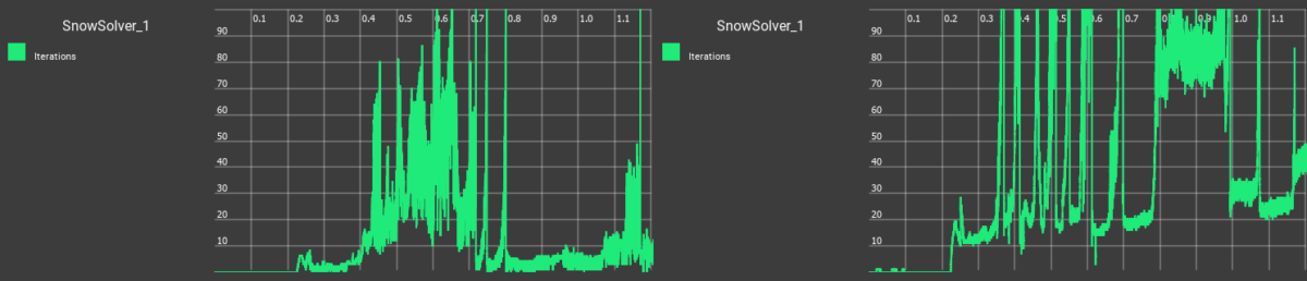
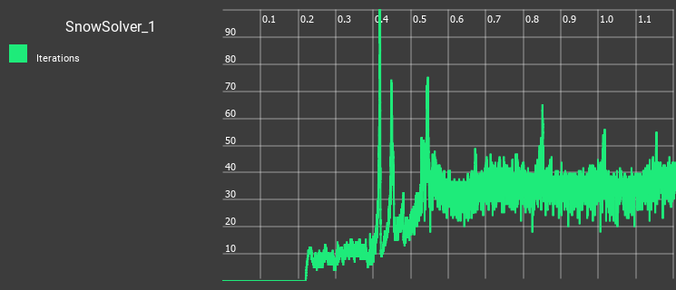
The guess that was used prior to PreonLab 5.0 is to just start with v^*. It consists of the velocity v^t of the previous timestep and all already known updated accelerations like gravity and airflows. It’s a good guess when the simulation is dominated by these forces, i.e. free-fall or wind-driven snow. It is also very good at keeping a simulation static: Any noisy accelerations created by the solver get overshadowed by gravity which presses the snow towards the rigid boundary.

Another method to obtain an initial guess is mentioned in Weiler et al.[2018]. It is used for the viscosity solver in PreonLab. In the snow solver, the idea is to reuse the change in velocity the solver had determined in the last timestep Δv=v^t−v^*. This change in velocity is the change in elastic acceleration the solver corrected in the last timestep. This guess assumes that the correction we applied in the last timestep stays the same. This guess is very good at propagating momentum through the snow medium. It also does not push particles towards the solid boundary by default. Solid boundaries can be a hard boundary condition to satifsy and are most likely to create the jumps in iterations we saw above.

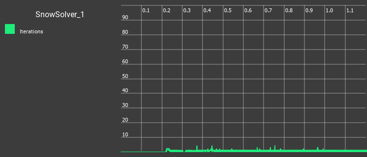
It would be nice to combine different guesses to play to their respective strengths and that’s precisely what we do. Gast et al. [2015] show that you can recast the equation solving problem (based on forces) as an optimization problem (based on energies). Energy is a scalar and should attain a minimum at the end of our solve. This makes energy a good measure to evaluate the quality of an initial guess. So we use minimization of energy as a guide to find an initial guess. Gast et al. [2015] proposes to do this decision each timestep globally for all particles. We deviate from this method and make each particle decide locally which method of initial guess is the best one for it. We do this by saying that each particle has a local energy: A particle goes through each guess and assumes all particles in its neighborhood move with the same guess. We evaluate the local energy for each guess. The particle then picks the guess with the lowest local energy. The cost of a single guess is close to half an iteration, so we can motivate doing two if we save one iteration.

How is our wedge doing with this idea?

Not bad at all. All the jumps but the first one are gone. The iterations look much more regular and are also down to 67% of the previous implementation which also reduces the runtime from 5h54m to 3h34m.

We made progress on both our challenges but we want to improve further. We have a linear system Av^t+Δ=v^*. This is a problem in itself that is well studied in numerical analysis. Depending on the mathematical properties of A different iterative schemes exist. The idea here now is that we want to solve an equivalent problem by preprocessing $A$ in such a way that it has nice properties (or technical: well-conditioned). Afterwards we recover the solution to our original problem. The equivalent problem we want to solve is the right preconditioned system:

$or$AP^-1 y = v^*

P needs to be easily invertible. Otherwise, we are solving two linear systems and gain nothing. A class of matrices that are easily invertible are diagonal matrices. The inverse of a diagonal matrix is diagonal as well. To find the inverse one just needs to apply the reciprocal to each diagonal entry. A common preconditioner is the Jacobi Preconditioner in which P is a diagonal matrix, and its diagonal entries are just the diagonal entries of A. The following picture (Source) illustrates how a preconditioning changes an optimization problem with S = AP^-1 :

A diagonal matrix is a very simple transformation matrix that only stretches/shrinks along the main axes as illustrated in the image. That way a Jacobi Preconditioner is helpful for a matrix $A$ that is diagonally dominant in the first place. The matrix P^-1 thus stretches and shrinks the space such that values scale similar along each axis.

Getting the diagonal for the Jacobi Preconditioner is not as simple as it sounds. Matrix-free methods like we use never explicitly form the matrix A but directly evaluate matrix-vector products Av. You can do the math to identify which calculations only contribute to the diagonal but we are not going to bother you with it. 

Of course during development of the new solver steps we ensured that our Jacobi Preconditioner is the right one and fits our matrix A. Additionally, we included automated tests in our test suite that verify this continuously to ensure that no code changes break the desired behavior.

What does this do for our wedge scene?

We improved massively and it shows in the runtime as well. We went from a scene that was very challenging to our solver to one that is not problematic at all anymore. Iterations are very low and stable, almost not improveable upon in the current scene. We totally crushed both the challenges we set for ourselves!

The wedge scene is of course not the only scene we improved upon: Our testing suite showed that our snow benchmarks also performed better. Scenes that are used in production were tested and showed massive improvements in stability and performance. This concludes our work on the snow solver for PreonLab 5.1. We hope that you had a good insight in how we, at FIFTY2, consistently challenge ourselves and are driven to come up with ideas to complete these challenges. Have fun with a snow solver that’s better than ever before!