PreonLab

Lid-driven Cavity (2D)

Validation objectives

The objective of the current work is to test the capabilities of PreonLab in capturing the behavior of 2-D flows inside confined volumes for different Reynolds numbers. Results are compared to the most widely used publication of this benchmark by Ghia et al. [1]

Problem description 

The problem consists of a fluid with density ρ and viscosity µ inside a square cavity. The cavity is made up of three rigid walls with no-slip conditions and length L as well as a no-slip lid which moves with a tangential velocity of U, see Fig. 1.

Benchmark quantities and target values

1. Visual comparison of time-averaged pathlines with those of literature [1]
2. Quantitative comparison of velocity profiles along the x- and y-centerlines with those from literature [1]

Test points

1. Reynolds number 100: lid velocity U = 1 m·s^-1, L = 1 m, ρ = 10 kg·m^-3, µ = 0.1 Pa·s
   a. spacing 10mm
   b. spacing 1mm
2. Reynolds number 1,000: lid velocity U = 1 m·s^-1, L = 1 m, ρ = 10 kg·m^-3, µ = 0.01 Pa·s
   a. spacing 10mm
   b. spacing 1mm
3. Reynolds number 10,000: lid velocity U = 1 m·s^-1, L = 1 m, ρ = 10 kg·m^-3, µ = 0.001 Pa·s
   a. spacing 10mm
   b. spacing 1mm
4. Reynolds number 100: lid velocity U = 10 m·s^-1, L = 1 m, ρ = 1 kg·m^-3, µ = 0.1 Pa·s
   a. spacing 10mm
5. Reynolds number 1,000: lid velocity U = 10 m·s^-1, L = 1 m, ρ = 1 kg·m^-3, µ = 0.01 Pa·s
   a. spacing 10mm
6. Reynolds number 10,000: lid velocity U = 10 m·s^-1, L = 1 m, ρ = 1 kg·m^-3, µ = 0.001 Pa·s
   a. spacing 10mm

In test points 1 to 3, viscosity is the variable to sweep Reynolds numbers. Moreover, in these test points, spacing is varied to test resolution independence of the results. In test points 4 to 6, lid velocity and density are changed compared to test points 1 to 3 for the respective Reynolds numbers in order to test parameter independence.

In PreonLab, simulations are performed in a transient manner. Therefore, the total kinetic energy of the fluid can be used as a parameter which determines whether the system has reached its steady state. The most important validation parameters used in the literature are horizontal velocity of the fluid, u, along the vertical centerline of the cavity as well as the vertical velocity, v, along the horizontal centerline of the cavity as illustrated in Fig. 1. Moreover, a visual comparison between the quasi steady pathlines obtained in PreonLab with the streamlines from [1] for test points 1 to 3 has also been carried out. Note that at steady state, streamlines and pathlines should look the same.

The results from PreonLab are compared against those provided by Ghia et al. [1] for three different Reynolds numbers 100, 1,000 and 10,000.

Test point 1 – Re = 100: U = 1 m·s^-1, ρ = 10 kg·m^-3, µ = 0.1 Pa·s

For the case with Reynolds number equal to 100, flow reaches its steady state at around 10s as can be seen from Fig. 2.

The time-averaged horizontal and vertical velocity values along the vertical and the horizontal centerlines are compared against those from [1] for particle spacings 10mm and 1mm and are depicted below, see Fig. 3. These values are averaged between 10s and 20s. Moreover, pathlines are compared to the streamlines obtained by Ghia et. al. [1], see Fig. 4.

Test point 2 – Re = 1,000: U = 1 m·s^-1, ρ = 10 kg·m^-3, µ = 0.01 Pa·s

For Re = 1,000, flow reaches its steady state after around 40s, see Fig. 5. The time span used for averaging velocity values is, therefore, between 50s and 60s.

Test point 3 – Re = 10,000: U = 1 m·s^-1, ρ = 10 kg·m^-3, µ = 0.001 Pa·s

At Re = 10,000, flow reaches its quasi-steady state after around 800s, see Fig. 8. Therefore, for the comparison with the reference article, the time span between 800s and 900s was used for time-averaging velocity values. As discussed in Sec.3, there are noticeable oscillations in the lid-driven cavity flows with high Reynolds numbers. Such oscillations can be observed in the PreonLab simulations. As stated in [6], these noticeable oscillations were not taken into account by Ghia et. al. [1].

In order to confirm that the flow pattern and the normalized velocity distributions are only dependent on the Reynolds number, three further simulations for the Reynolds number sweep are also performed for another combination of U and ρ. U is set to 10 m·s^-1 and ρ to 1 kg·m^-3. The resulting normalized velocity patterns are similar to those with the previous parameter set (U = 1 m·s^-1 and ρ = 10 kg·m^-3). The comparison between the simulation results using the second combination with those of literature are depicted below.

As in these test points the lid velocity is 10 m·s^-1, the normalized velocities have been defined for the comparisons which are u_norm = u/U = u/10 and u_norm = v/U = v/10.

Test point 4 – Re = 100: U = 10 m·s^-1, ρ = 1 kg·m^-3, µ = 0.1 Pa·s

Test point 5 – Re = 1,000: U = 10 m·s^-1, ρ = 1 kg·m^-3, µ = 0.01 Pa·s

Test point 6 – Re = 10,000: U = 10 m·s^-1, ρ = 1 kg·m^-3, µ = 0.001 Pa·s

The lid-driven cavity problem is of high importance in fluid dynamics serving as a benchmark for the validation of numerical methods as well as for studying fundamental aspects of incompressible flows in confined volumes driven by the tangential motion of one or more bounding walls. The numerical computation of two-dimensional cavity flows requires little resources making it an efficient test bed for numerical codes and for studying pure two-dimensional flow physics.

The quest for efficiency and accuracy began with the work of Ghia et al. [1] in 1982. Their study covered steady-state two-dimensional flow for Reynolds numbers up to 10,000 in a square lid-driven cavity with its moving wall having constant velocity. This article is still the most widely used reference for this regard. Therefore, in the current article, PreonLab is validated for Reynolds number equal to 100 and 1,000 as well as 10,000 against the results from this article.

Typical streamline patterns of the two-dimensional lid-driven cavity for Reynolds numbers 1, 100, 1,000 as well as 10,000 are shown in Fig. 14. For Re = 1, the streamlines are nearly symmetrical, due to the symmetry of velocity field in the Stokes-flow limit where Re → 0. Two separated eddies in the bottom corners are characterized by the two separating streamlines. When the Reynolds number becomes large (Re = 10,000), inertia terms in the Navier-Stokes Equation become dominant and destroy the reflectional symmetry of the velocity field with respect to x = 0. The separated vortices at the bottom become stronger, and even a second separated vortex is generated in the bottom right corner of the cavity. Moreover, a third separated region is created, for Reynolds numbers greater than 1,000, close to the upstream corner of the moving lid near (Look at the case with Re = 10,000). For even higher Reynolds numbers, the core of the vortex approaches a solid-body rotation with circular streamlines and constant vorticity [5].

It should be noted that while the two-dimensional flows for small and moderate Reynolds numbers become steady at some point in time, flows with higher Reynolds numbers (dominating inertial forces) undergo a so-called Hopf bifurcation and become time-dependent which was not taken into account by Ghia et al. as reported in [6]. The critical Reynolds number regarding this effect, however, varies somewhat among different investigations for this purpose based on the numerical methods used. Further information can be obtained from [6] to [12].

In this study, PreonLab has been successfully validated for a 2-D lid driven cavity flow across Reynolds numbers ranging from 100 to 10,000 for different combinations of viscosity, density and lid velocity. The results are in good agreement with those presented by Ghia et al. [1] for a particle resolution of 10mm. Furthermore, it has been shown that varying the particle resolution by an order of magnitude only marginally affects the quality of the results as expected. This means that the computed velocity fields are matching the expected flow fields for the respective Reynolds numbers. Furthermore, while for the low Reynolds number of 100, both coarse and fine resolutions show almost no difference, small deviations between the resolutions can be observed for higher Reynolds numbers, particularly 10,000. These small deviations, however, are explained by the coarse resolution of 10mm not capturing the turbulent flow as with a particle spacing of 1mm. Thus, it can be concluded that the Preon solver shows convergent behavior.

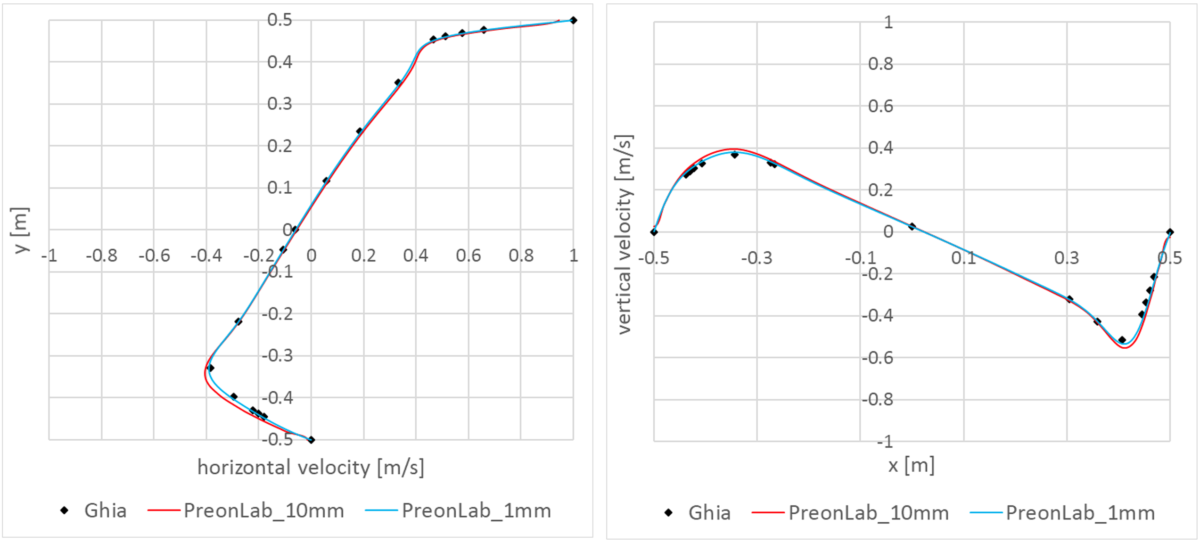
[1] Ghia, U. K. N. G., Ghia, K. N., & Shin, C. T. (1982). High-Re solutions for incompressible flow using the Navier-Stokes equations and a multigrid method. Journal of computational physics, 48(3), 387-411.

[2] Santhosh Kumar, D., Suresh Kumar, K., & Kumar Das, M. (2009). A fine grid solution for a lid-driven cavity flow using multigrid method. Engineering Applications of Computational Fluid Mechanics, 3(3), 336-354.

[3] Poochinapan, K. (2012). Numerical implementations for 2D lid-driven cavity flow in stream function formulation. ISRN Applied Mathematics, 2012.

[4] Kuhlmann, H. C., & Romanò, F. (2019). The lid-driven cavity. In Computational Modelling of Bifurcations and Instabilities in Fluid Dynamics (pp. 233-309). Springer, Cham.

[5] Batchelor, G. K. (1956). On steady laminar flow with closed streamlines at large Reynolds number. Journal of Fluid Mechanics, 1(2), 177-190.

[6] Shen, J. (1991). Hopf bifurcation of the unsteady regularized driven cavity flow. Journal of Computational Physics, 95(1), 228-245.

[7] Auteri, F., Parolini, N., & Quartapelle, L. (2002). Numerical investigation on the stability of singular driven cavity flow. Journal of Computational Physics, 183(1), 1-25.

[8] Nobile, E. (1996). Simulation of time-dependent flow in cavities with the additive-correction multigrid method, part II: applications. Numerical Heat Transfer, 30(3), 351-370.

[9] C.-H. Bruneau and M. Saad. The 2d lid-driven cavity problem revisited. Comp. Fluids, 35:326–348, 2006.

[10] Poliashenko, M., & Aidun, C. K. (1995). A direct method for computation of simple bifurcations. Journal of Computational Physics, 121(2), 246-260.

[11] Fortin, A., Jardak, M., Gervais, J. J., & Pierre, R. (1997). Localization of Hopf bifurcations in fluid flow problems. International Journal for Numerical Methods in Fluids, 24(11), 1185-1210.

[12] Sahin, M., & Owens, R. G. (2003). A novel fully‐implicit finite volume method applied to the lid‐driven cavity problem—Part II: Linear stability analysis. International journal for numerical methods in fluids, 42(1), 79-88.