Analysis of a 3-D Breaking Dam Flow Using Single Phase Particle-based (SPH) Simulations

August 12, 2022
Siddharth Marathe

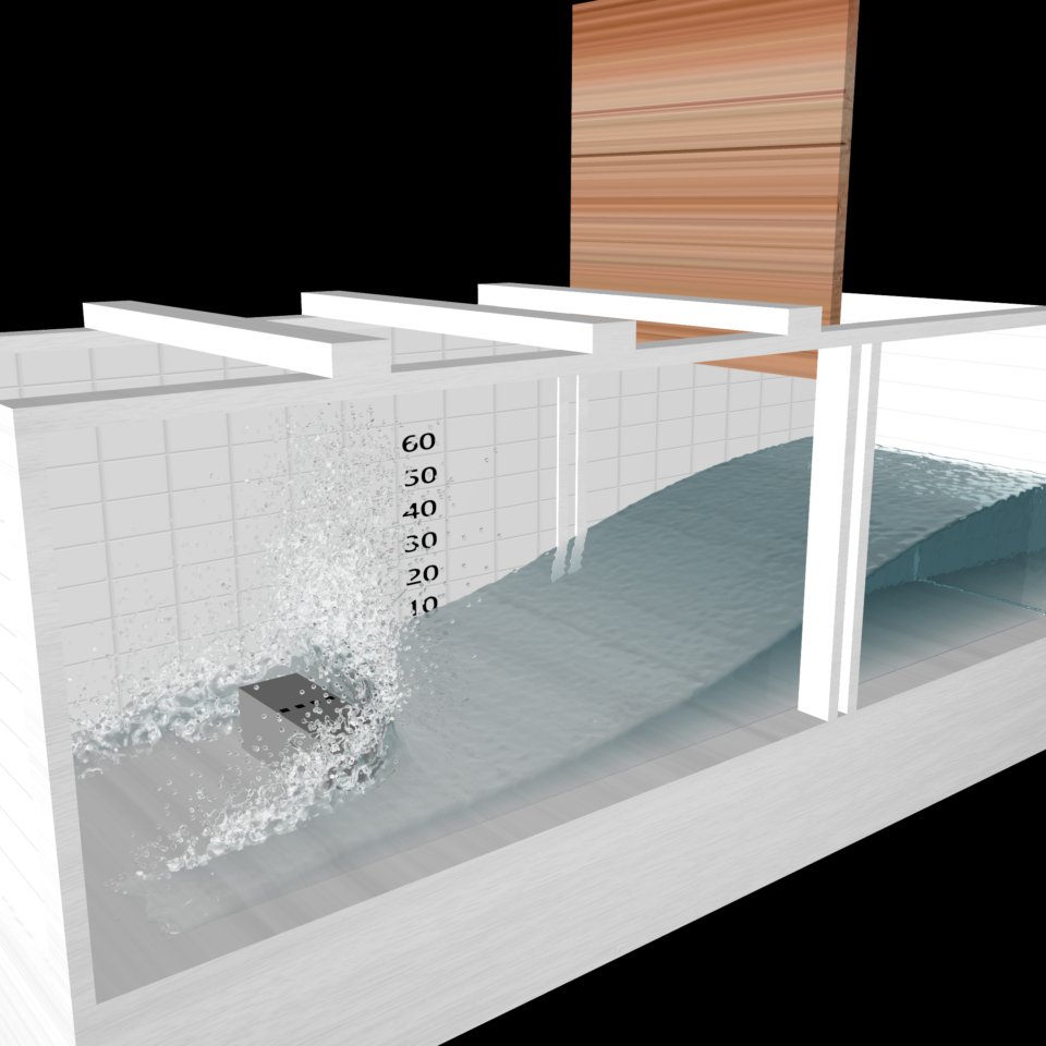
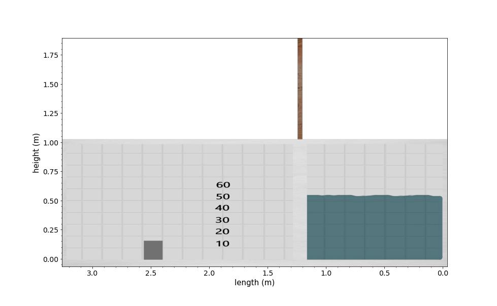
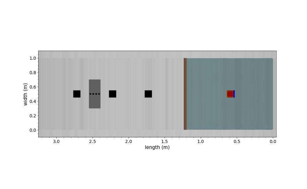
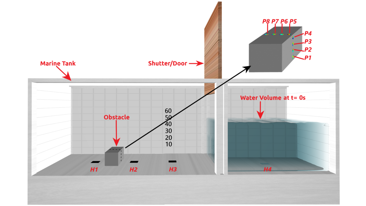
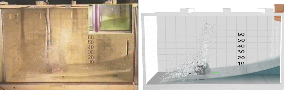
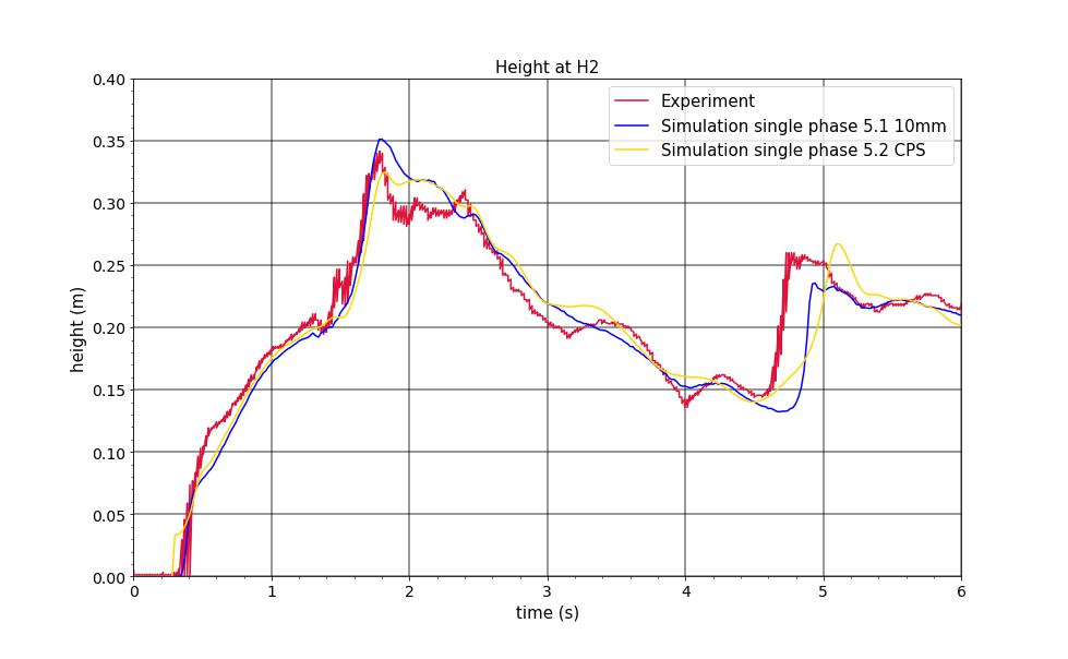
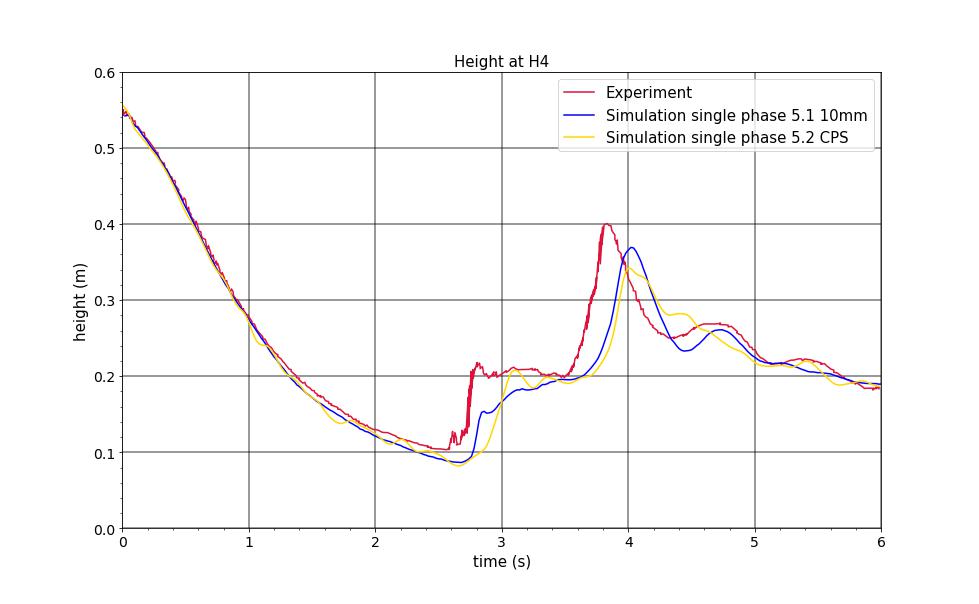
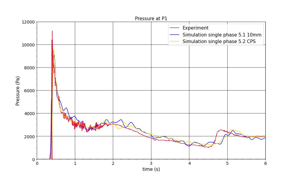
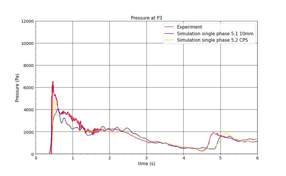
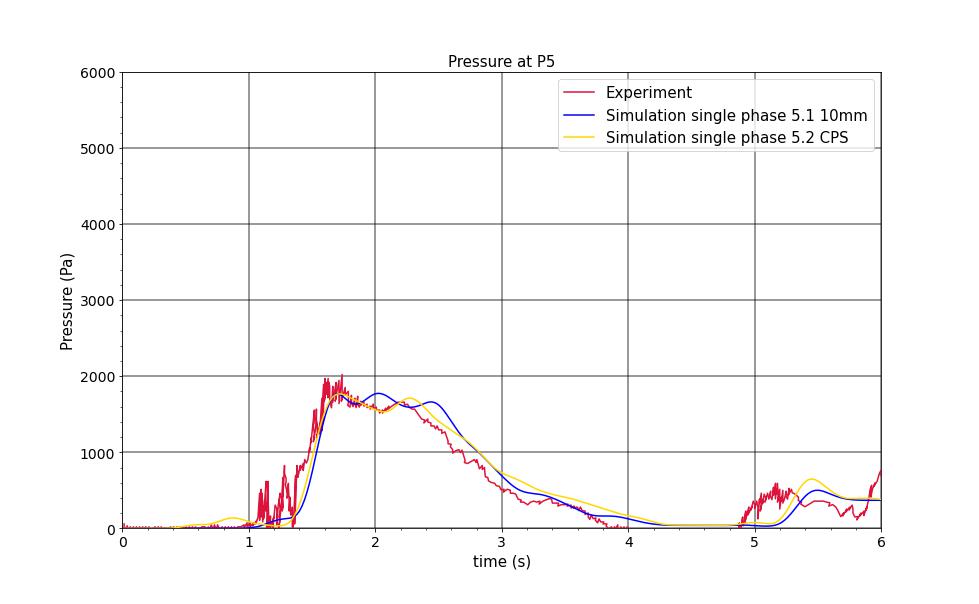
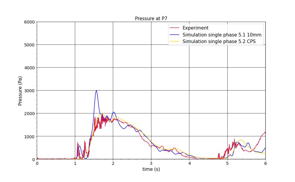
In this article, we look at an application from the maritime industry for a breaking dam flow and the wave impact on an obstacle placed in the flow. Initially, a series of uniform resolution simulations were performed with PreonLab 5.1 to determine the particle size necessary for accurate simulation results.
Subsequently, simulations have also been performed with PreonLab 5.2 to make use of the new Continuous Particle Size (CPS)
feature and analyze the benefits this feature provides towards reducing computational effort without compromising on the accuracy of the results.
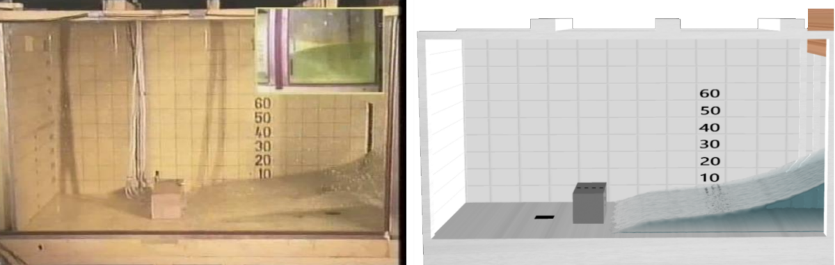
The simulation results obtained in PreonLab are compared qualitatively and quantitatively with experiment results published in the paper by Kleefsman et.al [1].
The experiments were performed at the Maritime Research Institute Netherlands (MARIN). All the experimental data generated is also available to download from the ERCOFTAC database [2].

Share:

Setup in PreonLab

The geometrical setup used for the simulation is shown in Figures 1a and 1b. The marine tank is a cuboid with the dimensions 3.22 m x 1 m x 1 m and has an open roof.
A volume of water 1.22 m x 1 m x 0.55 m is generated at the right bottom corner (Figure 1a) of the marine tank at t = 0 s.
A cuboid-shaped obstacle, representing a container on the deck of a ship, with dimensions
0.16 m x 0.4 m x 0.16 m is placed along the centerline about 1.2 m away from the volume of water. The details of the setup are shown in Figure 2.
Figure 1a: Side view showing the length and height dimensions of the marine tank.
Figure 1b: Top view showing the length and width dimensions of the marine tank.
Figure 2: Marine tank setup.

According to [1] , the shutter holding the volume of water in place is pulled up almost instantaneously before the water flows across the tank. The influence of varying shutter opening speeds is not investigated with this setup. Hence, the wooden shutter included in the setup in PreonLab (Figure 2) serves rendering purposes alone and has no influence on the simulation. It is assumed that the shutter is opened instantaneously, and that the volume of water breaks down into a flow due to gravity.
Four height sensors (H1, H2, H3 and H4) are placed along the floor of the marine tank and 8 force sensors (P1 – P8) are placed along the surface of the obstacle to measure pressure, matching the measurement locations described in the experimental setup. The sensors have the dimensions
20 mm x 20 mm.

Overview Simulations

The simulations were run on 1 CPU with 8 cores. The following table gives an overview of the simulation times required for each investigated variant.

Nr.
1
Particle Size
40 mm
Refinement
uniform
   Max No. of     Particles
10,433
    Simulation        Time on
       8 Cores
1 min
    PreonLab       Version
5.1
Nr.
2
Particle Size
20 mm
Refinement
uniform
   Max No. of     Particles
84,231
    Simulation        Time on
       8 Cores
7 min
    PreonLab       Version
5.1
Nr.
3
Particle Size
10 mm
Refinement
uniform
   Max No. of     Particles
675,036
    Simulation        Time on
       8 Cores
1 hr 40 min
    PreonLab       Version
5.1
Nr.
4
Particle Size
40 mm
    to
10 mm
Refinement
Continuous    Particle       Size
   Max No. of     Particles
357,240
    Simulation        Time on
       8 Cores
56 min
    PreonLab       Version
5.2

The simulation with particle size 40 mm runs in one minute (1 min 7 s) using 8 cores of processing power. While the general behavior of the flow matches the qualitative results from the experiment quite well, the quantitative results for height and pressure are not accurate enough.
This happens, since the particle size (40 mm) is too large compared to the dimensions of the sensors (20 mm x 20 mm). A similar problem occurs when the particle size is reduced to 20 mm,
although a marked improvement in the calculated pressure can be observed. Increasing the resolution to 20 mm results in an increase in the number of particles in the simulation and thereby an increase in the total simulation time – as can be seen from the table above.
The simulation variant with a uniform particle size of 10 mm requires about one hundred minutes to reach completion, however, the accuracy of the results improves drastically. These results have been compared with the measured values from the experiment in Figures 5a-5f.

Using CPS, the particle size was then reduced only in the region of interest i.e., a volume around the obstacle, so that the sensors can accurately capture information about the flow characteristics. As a result, the total number of particles and consequently the computational time reduced significantly (compared to the uniform resolution simulation with particle size
10 mm).

It should be noted that a portion of the computational power is required for performing the splitting and merging of particles when using CPS. However, we are able to achieve results with an accuracy, which is similar to that when a uniform resolution with particle size = 10 mm is used – with only about half of the computational time required for simulation.
This shows that CPS can be effectively applied to cases such as the breaking dam flow, by keeping the particle size large for the bulk of the flow and reducing the particle size in the regions which need to be investigated closely.

Setup with CPS

An initial particle size of 40 mm is selected for the simulation performed with PreonLab 5.2. Using CPS, the particle size is reduced to 10 mm in the region of interest. In the following video, the breaking dam flow has been visualized in a manner such that the different particle sizes can be observed:

Please agree to the transfer of data to third parties as set out in our privacy policy.

Wave Impact Video with Continuous Particle Size (CPS).

The smaller particles within the refinement domain are color-coded white, while the larger particles are color-coded blue. Particles with a particle size between 40 mm and 10 mm are color-coded green.

Qualitative comparison of results

Figures 3 and 4 show a qualitative comparison between the breaking dam flow simulated with PreonLab and snapshots from the experiment [1] at 0.4 s and 0.56 s, respectively:

Figure 3: Snapshot of the dam break simulation (right) compared with the experiment (left) at time 0.4 s.

Figure 4: Snapshot of the dam break simulation (right) compared with the experiment (left) at time 0.56 s.

The following video showcases the breaking dam flow with a box-shaped obstacle in the flow simulated with PreonLab for a total of 6 seconds (simulated flow from the uniform resolution simulation has been used for rendering purposes).

Please agree to the transfer of data to third parties as set out in our privacy policy.

3-D simulation of a breaking dam flow with a box-shaped obstacle in the flow.

Quantitative Results

The flow simulated with PreonLab is quantitatively compared with the measured data by analyzing the water height at 2 locations in the tank (H2 and H4), and the pressure exerted by the water at 4 locations (P1, P3, P5 and P7) on the obstacle, corresponding to the results published in [1].

Note: The measured values for pressure at P1, P3, P5 and P7 published in [1] show an initial value of 1000 Pa acting on the obstacle – even at t = 0 s, where the flow has not reached the obstacle. Since no direct explanation for this pressure value could be found in the paper, this offset of
1000 Pa was deducted from the experiment data used for the comparisons in the following figures.

Figure 5a: Height in (m) after 6 s of simulation at location H2: Comparison between simulation results using a uniform resolution, simulation results using CPS and experimental data.

Figure 5b: Height in (m) after 6 s of simulation at location H4: Comparison between simulation results using a uniform resolution, simulation results using CPS and experimental data.
Figure 5c: Pressure in (Pa) after 6 s of simulation at location P1: Comparison between simulation results using a uniform resolution, simulation results using CPS and experimental data.
Figure 5d: Pressure in (Pa) after 6 s of simulation at location P3: Comparison between simulation results using a uniform resolution, simulation results using CPS and experimental data.
Figure 5e: Pressure in (Pa) after 6 s of simulation at location P5: Comparison between simulation results using a uniform resolution, simulation results using CPS and experimental data.
Figure 5f: Pressure in (Pa) after 6 s of simulation at location P7: Comparison between simulation results using a uniform resolution, simulation results using CPS and experimental data.

All the quantitative results show an overall good agreement with the experiment results. A slight delay can be observed with the simulated data around 4 s at height sensor H4 and between 4.5 s and 5 s at height sensor H2 as well as at the pressure sensors. This possibly occurs due to minor differences in the simulated wave propagation between two simulation time steps which are prominently visible due to getting accumulated towards the later part of the simulation. Similar delays can also be observed with the original simulation results by [1].

Conclusion

The results presented in this article showcase the capabilities of PreonLab for investigating free surface flows.
Using CPS, the computational effort can be kept to a minimum without compromising
on the accuracy of the results in the region of interest.

References

[1] K. M. T. Kleefsman, G. Fekken, A. E. P Veldman, B. Iwanowski, and B. Buchner, A Volume-of-Fluid based simulation method for wave impact problems. J. Comp. Phys., 206:363–393, 2005
doi:10.1016/j.jcp.2004.12.007 (rug.nl)

[2] SPH European Research Interest Community SIG, R.Issa and D. Violeau, Test-Case 2 3D dam breaking, Test 02 (spheric-sph.org)

RELATED ARTICLES

LEARN MORE ABOUT PreonLab Updates

How to get started with
Preonlab CFD software?
Get in Touch