Thermal Conduction within a Rod

March 03, 2022
Loïc Wendling

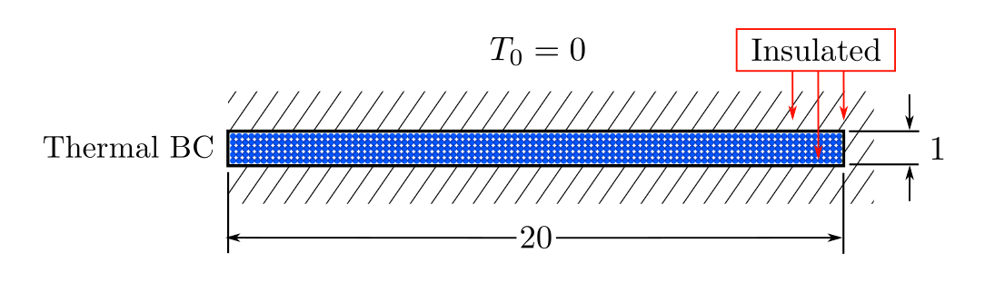
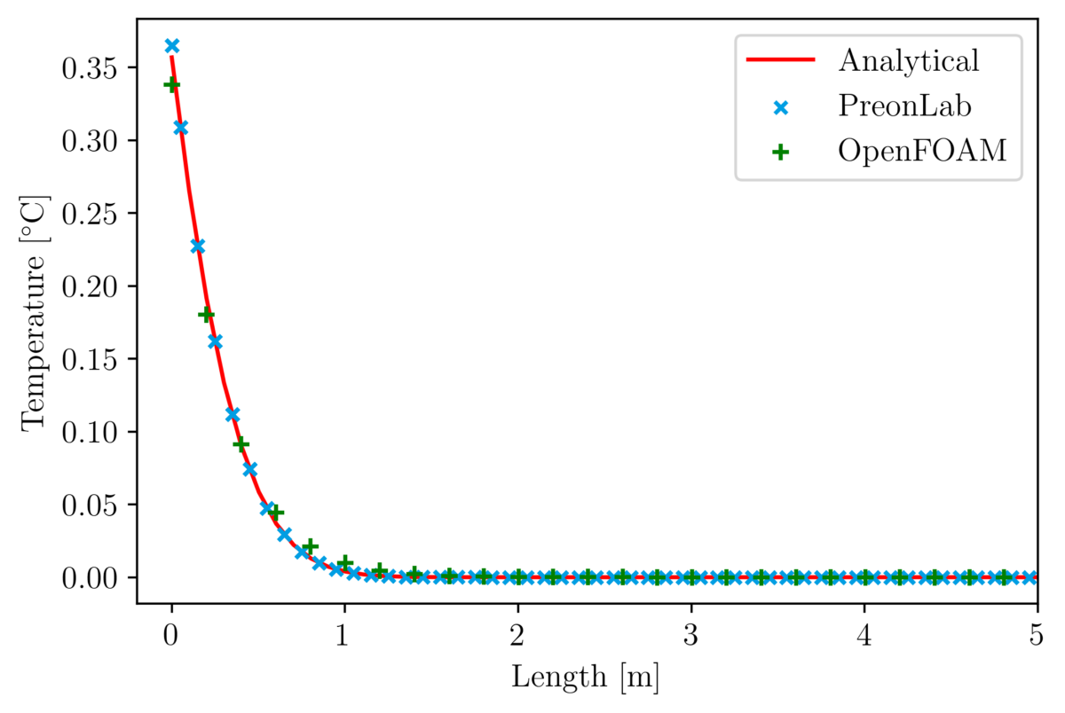
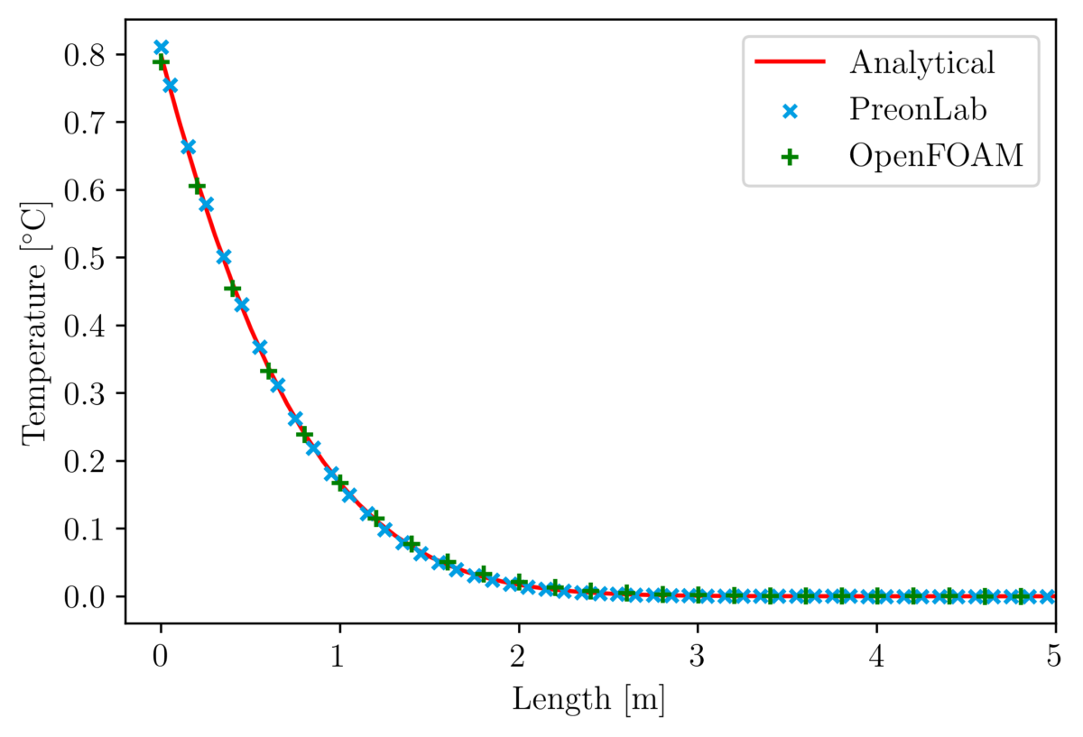
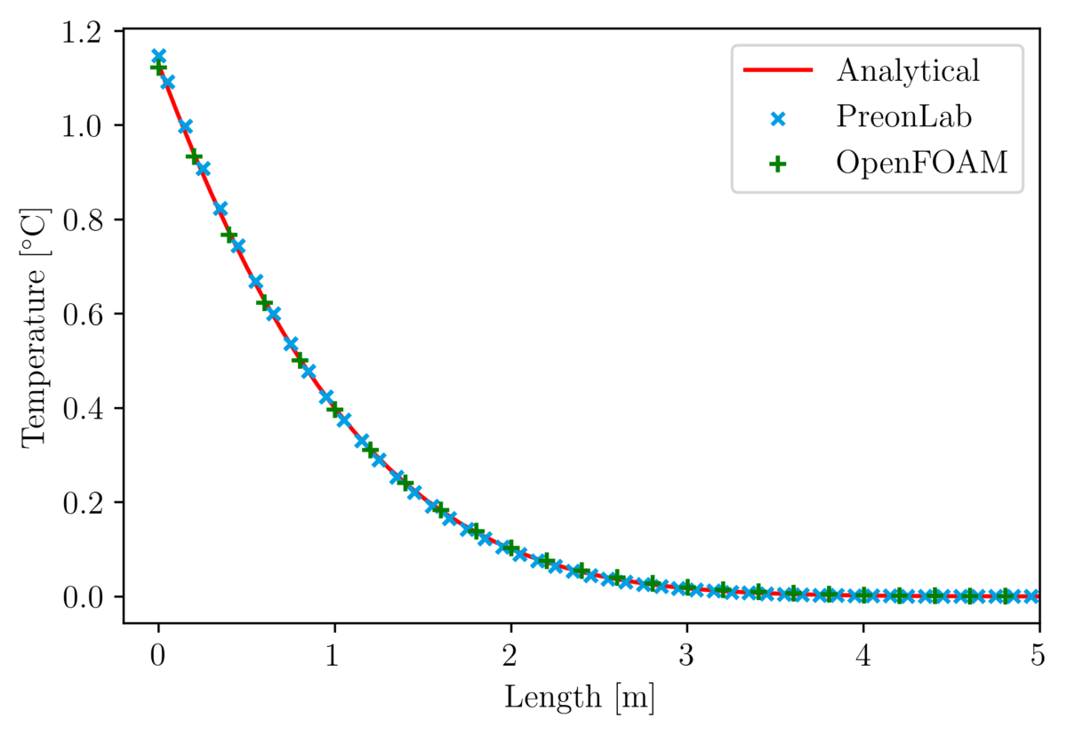
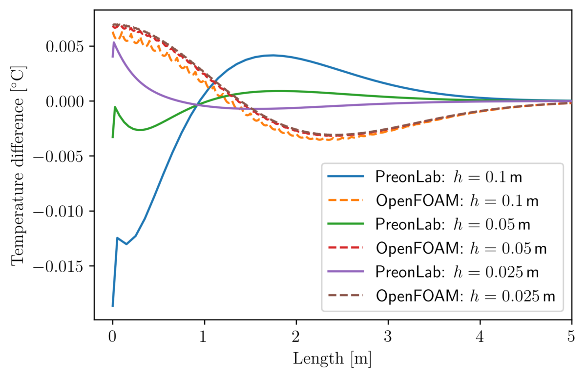
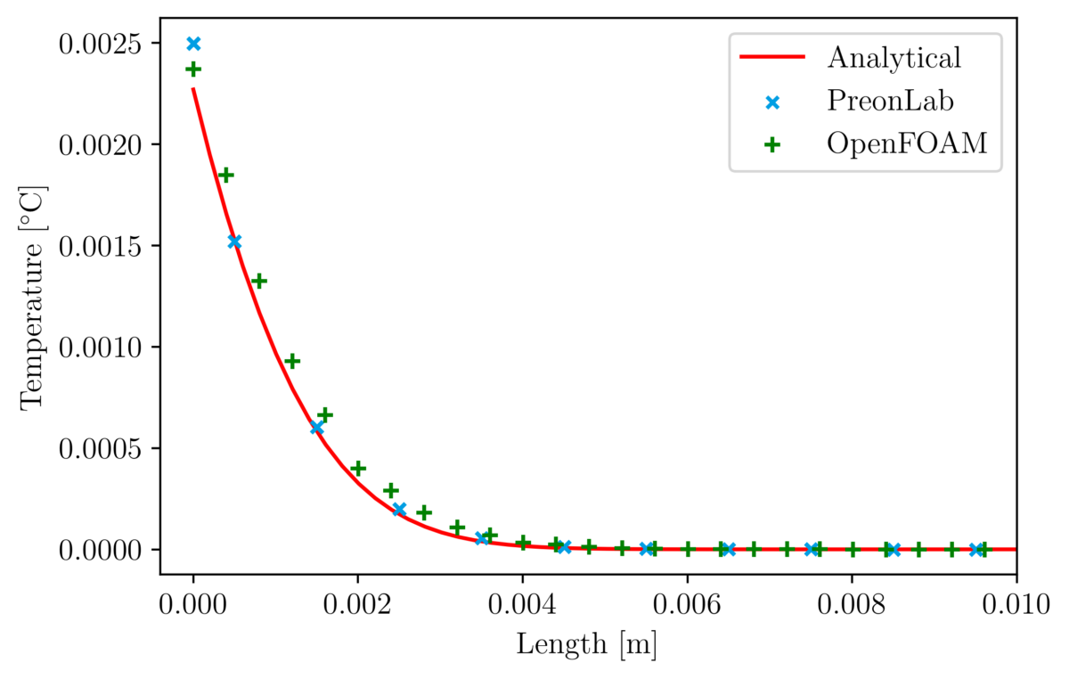
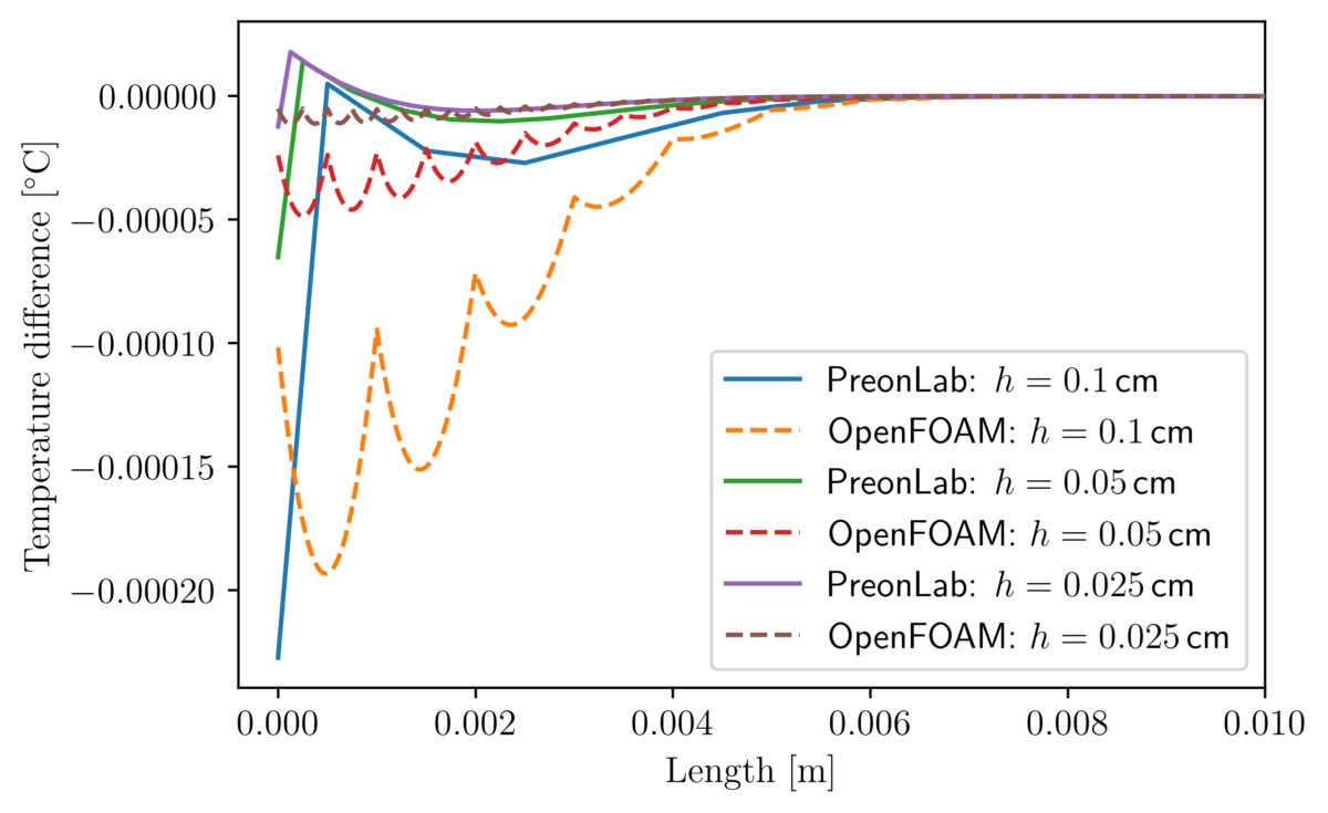
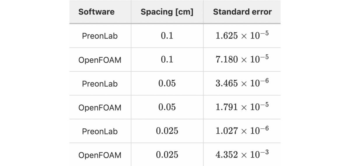
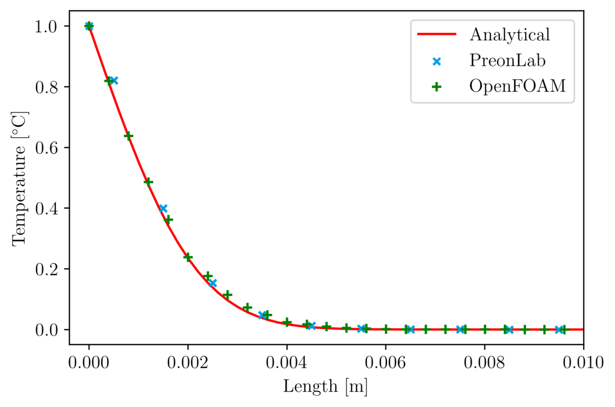
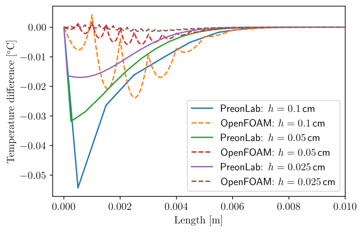
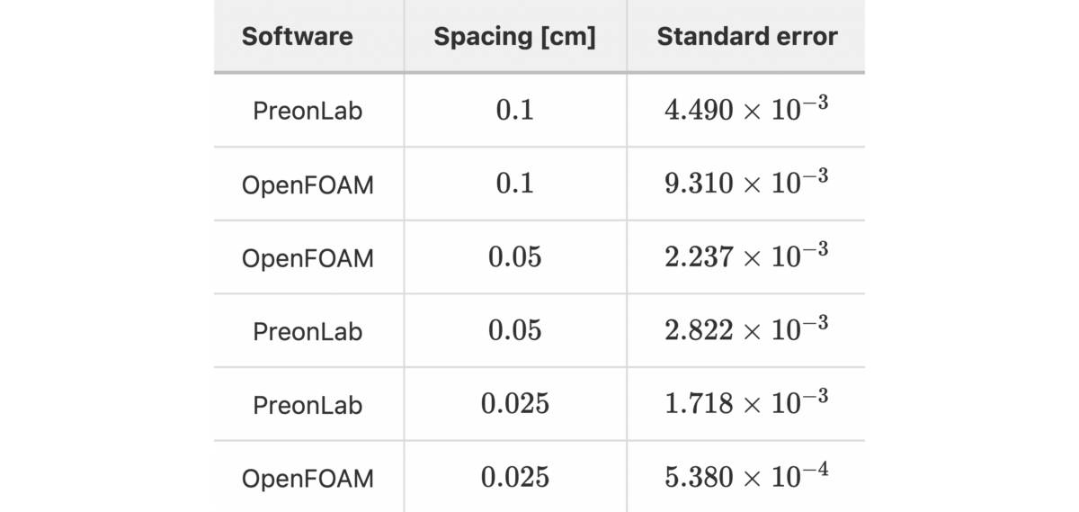
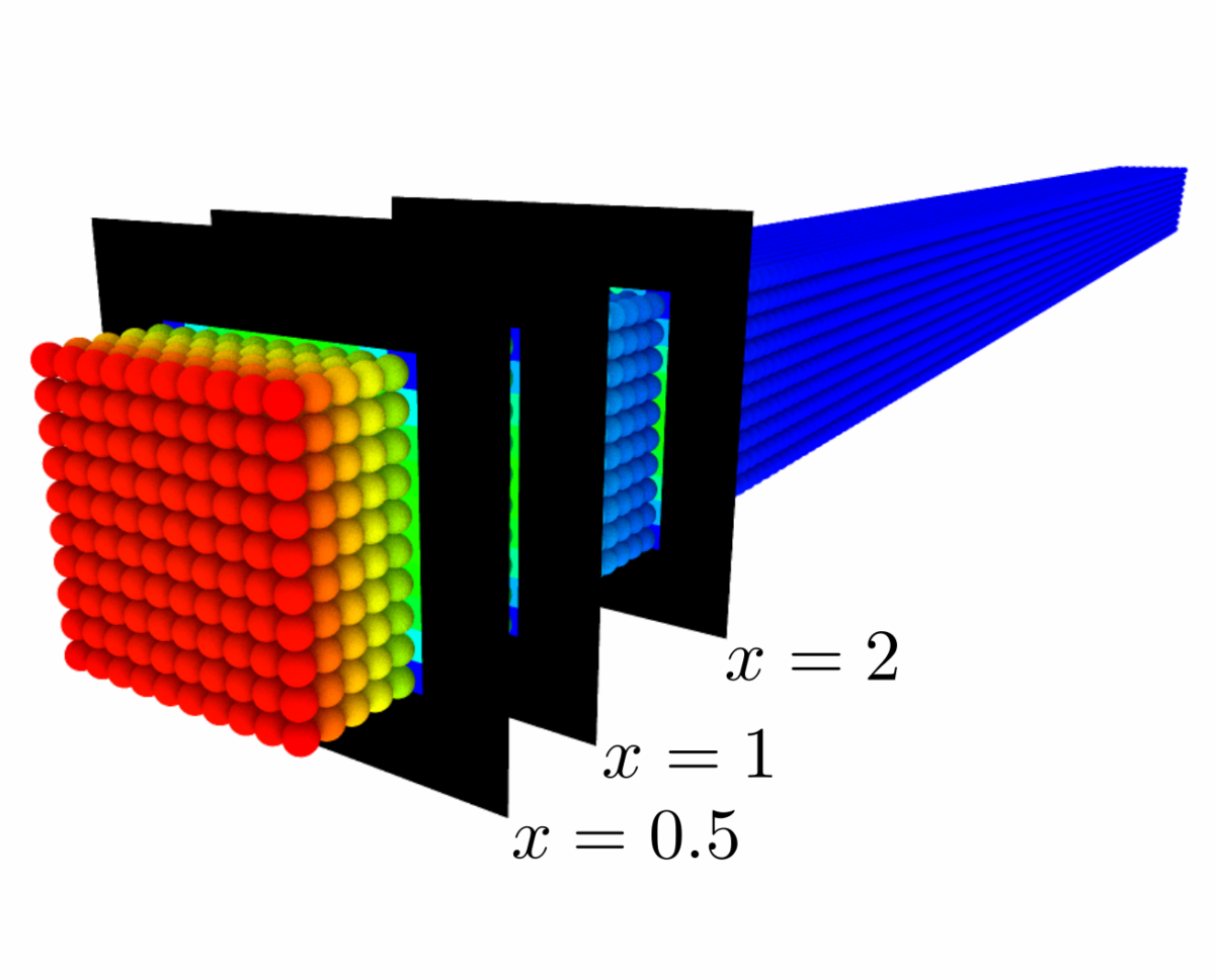
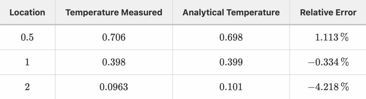
Thermal validation benchmarks are great tools to build confidence in thermal solvers. The rod conduction benchmark is useful to check that conduction phenomena are accurately simulated. In this article, the results from various configurations of the rod conduction benchmark will be presented alongside a thorough comparison with the popular CFD code OpenFOAM.

Share:

Introduction

Solver validation is an important aspect of product development and it is achieved by finding relevant benchmarks that build confidence in the solver. The thermal solver in PreonLab is a vital component for numerous applications from pipe flows to impinging jets. The rod conduction benchmark [1] is chosen to validate conduction phenomena. The benchmark having an analytical solution and being simple to simulate, multiple variations can be studied to test the limit of the thermodynamic implementation. Different types of thermal boundaries, solver types, and sensor plane locations are investigated.

Method

The goal is to validate the implementation of the transient heat equation within PreonLab. This solver leverages the implicit Smoothed Particle Hydrodynamics implementation and the efficient data structures available for the fluid solver. The strong form of the heat equation reads:

where T, t, and α are respectively the temperature field, the time, and the thermal diffusivity. The thermal diffusivity is defined as:

where α, k, ρ, and Cp are respectively the thermal diffusivity, the thermal conductivity, the density, and the heat capacity. The same heat equation is also solved with the popular finite volume solver OpenFOAM where the LaplacianFoam solver is used.

Setup

This test case is composed of a long rod made of isotropic material with a heat source applied on one side. Over time, the heat diffuses within the medium. The setup and key dimensions are presented in Figure 1. When simulating water material properties, the domain is scaled down a hundred times to compensate for the comparatively low conductivity (the rod is 20cm long and 1cm wide). The original 1D analytical setup is expanded to 3D in the simulation but the analytical solution still holds along the length of the 3D rod. The initial temperature field is initialized to zero.

Figure 1: Setup of the benchmark. “Thermal BC” is the thermal boundary condition which is either temperature or heat flux boundary condition.

Two material properties are considered: unity and water. The unity material properties are used to simplify the computation and remove all dependency on the material properties for the resolution of the heat equation. The detailed material properties are listed in Table 1.

Table 1: Material properties used.

The two main thermal boundary condition types are considered:

  • Heat flux boundary: W/m2
  • Temperature boundary: = 1°C

For simplicity, the thermal boundary conditions are set to one.

Analytical Solution

The temperature along the centerline is governed by an analytical solution that depends on the type of thermal boundary condition applied on the side of the rod. The models can be found in the work of Cengel and Ghajar [1]. When using a heat flux boundary condition the analytical solution reads:

where T0, t, and x are respectively the initial temperature, the time, and the position along the rod. When using a temperature boundary condition the analytical solution reads:

where Ts is the temperature boundary condition. The advantages of these analytical models are that they can be adapted to different material properties for testing and that the solution at all times and all positions can be obtained.

Results

The various cases are summarized in table 2. During testing in PreonLab, the fluid and solid solvers have been used and did not show any discrepancy between them.

Table 2: The different variants considered.

Unity Material

The simplified unity material will be analyzed first.

Case 1 – Heat Flux Boundary Condition

The heat flux boundary condition is a Neumann type boundary condition where the user can control the temperature gradient applied on the computational domain. In this case, the temperature on the hot wall is measured using a thermal sensor object. The resulting temperature distribution in PreonLab is rendered in Figure 2. The left side of the rod has the highest temperature and then it monotonically decreases along the length of the rod. The transient solution for the heat flux boundary condition is presented in Figures 3-5. Even the greater non-linearity observed early at 0.1s is captured properly. In all cases, PreonLab is in good agreement with the analytical solution and with OpenFOAM. Figure 6 shows the temperature difference between the simulation and the analytical solution for various spacings (h). As the spacing is reduced, the error reduces as well. The numerical errors in PreonLab and OpenFOAM are very close as shown in Table 3.

Figure 2: Temperature distribution within the rod at 1 sec.

Figure 3: Temperature distribution along the centerline at 0.1 sec.

Figure 4: Temperature distribution along the centerline at 0.5 sec.

Figure 5: Temperature distribution along the centerline at 1 sec.

Figure 6: Temperature difference between the analytical solution and the simulation results along the centerline at 1 sec.

The standard deviation, σ, is computed for this test case as follows:

where N, Tsim,i , and Tth,i are respectively the number of datapoint along the centerline of the rod, the simulation temperature at point i, and the theoretical temperature at point i. Table 3 presents the standard error for the simulations of this section.

Table 3: Standard deviation for the unity material and heat flux boundary condition at 1 sec.

Case 2 – Temperature Boundary Condition

The other type of thermal boundary condition is a temperature boundary condition where the temperature is directly set on the side of the rod. In this configuration, the maximal temperature in the domain will be one and only the temperature within the domain will change over time. These types of boundary conditions are referred to as Dirichlet boundary conditions. The temperature along the centerline of the rod for PreonLab and OpenFOAM is presented in Figure 7. Very good agreement between the solvers and the analytical solution can be again observed. For a more detailed comparison, the temperature difference between simulation and analytical for the two solvers and various spacing are plotted in figure 8 and show a similar error. The simplest material property model is now verified and a more realistic model can now be investigated.

Figure 7: Temperature distribution along the centerline at 1 sec.

Figure 8: Temperature difference between the analytical solution and the simulation results along the centerline at 1 sec.

Table 4: Standard deviation for the unity material and temperature boundary condition at 1 sec.

Water Material

Because water is such a ubiquitous material, it is the default material property used in PreonLab. The heat flux and temperature boundary conditions will be tested again with this material.

Case 3 – Heat Flux Boundary Condition

Water follows a similar trend to the unity material. The non-linearity in the temperature field is well captured by PreonLab.

Figure 9: Temperature distribution at 1s.

Figure 10: Temperature difference between the analytical solution and the simulation results.

Table 5: Standard deviation for the water material and heat flux boundary condition at 1 sec.

Case 4 – Temperature Boundary Condition

The last variation is using water with a temperature boundary condition. The temperature distribution and temperature difference are plotted in Figures 11 and 12 respectively. PreonLab is also validated for this case.

Figure 11: Temperature distribution at 1 sec.

Figure 12: Temperature difference between the analytical solution and the simulation results at 1 sec.

Table 6: Standard deviation for the water material and temperature boundary condition at 1 sec.

Sensor planes

Finally, the thermal sensor will be also tested to make sure that the reported temperature is correct. To achieve it multiple sensor planes are added to Case 1 along the centerline to measure the temperature at various points (cf. Figure 13). The analytical model is used to evaluate the relative error of the simulation result at 1 second. The values are summarized in Table 7.

Figure 13: Position of the thermal sensors.

Table 7: Summary of the results from the sensor planes placed along the centerline at 1 sec.

Conclusion

In conclusion, PreonLab passed the rod conduction benchmark for a wide variety of configurations, different materials, different thermal boundary conditions, and different spacings. No discrepancy between the fluid and solid solvers in PreonLab has been observed. Thanks to the available analytical solutions, this benchmark has been proven to be fast and accurate to validate thermal conduction. The analytical solutions available can be adapted to more material properties. Each variation shows very good agreement with the analytical solution for both PreonLab and OpenFOAM. The sensor plane has also proven reliable for checking the temperature at specific points.

Bibliography

[1] Cengel, Y., and Ghajar, A. Heat and Mass Transfer: Fundamentals and Applications. McGraw-Hill Education, 2010.

RELATED ARTICLES

LEARN MORE ABOUT PreonLab Updates

How to get started with
Preonlab CFD software?
Get in Touch