Conduction Through a Composite Wall

April 28, 2022
Loïc Wendling

In this test case, the thermal conduction through a wall made of multiple materials is analyzed. The analytical solution of the benchmark found in Lewis et al. [1] will be used to validate the thermal conduction and Conjugated Heat Transfer (CHT) in PreonLab. Furthermore, different thermal boundary conditions and the heterogenous spacing feature that allows you to choose different spacings for each solver are tested as well.

Share:

Setup

The composite wall intended here is composed of one or more layers of material with different conductivities. An example can be seen in Figure 1. The geometry of a wall is interesting here because when it is assumed that the whole sides of the wall are heated uniformly, the temperature changes only in the direction normal to the wall. At steady-state, the analytical temperature profile depends only on the wall depth \(x\), and the heat flux at each location along the wall is constant due to the conservation of energy. Thus, having different thermal conductivities for each layer leads to different temperature gradients for each of them. An example of the resulting temperature distribution through the wall can be seen in red in Figure 1. Because the analytical solutions are for steady-state, the transient simulation is run until there are no more changes in the temperature field.

Figure 1: Heat conduction in a composite wall. The red line is an example of temperature distribution.

At steady-state, the heat flux in the wall reads:
$$ Q = -\frac{k_1 A}{x_1} \left(T_2 – T_1 \right) = -\frac{k_2 A}{x_2} \left(T_3 – T_2 \right) = -\frac{k_3 A}{x_3} \left(T_4 – T_3 \right) \hspace{1.5cm}(1)$$

After rearranging:
$$ Q = \frac{(T_1 – T_4)}{\left[ \frac{x_1}{k_1 A} + \frac{x_2}{k_2 A} + \frac{x_3}{k_3 A}\right]}\hspace{1.5cm}(2) $$

Where:

  • \(Q\): heat flux
  • \(T_1\) to \(T_4\): temperatures at the interfaces of the layers.
  • \(x_1\) to \(x_3\): thicknesses of each layer of the wall
  • \(k_1\) to \(k_3\): thermal conductivity of each layer
  • \(A\): surface area at the boundaries.

The user can set either heat flux or temperature boundary conditions on the boundaries of the wall. Both configurations are investigated. In PreonLab when using at least two layers two solvers are required and they interact forming a Conjugate Heat Transfer (CHT) setup.

Cases

Various cases are considered from the easiest to the more complex. For all cases the surface area \(A\) will be taken as \(1\) m\(^2\) (the domain is a cube of size \(1\) m). The percentage given after a result is the relative error.

Case 1 – 1 Layer

The most simple configuration is one layer made of one material as shown in Figure 2.

Figure 2: Setup for case 1.

Using equation 1, the heat flux can be estimated for this configuration with: $$ Q = -\frac{k_1 A}{x_1} \left(T_2 – T_1 \right)\hspace{1.5cm}(3) $$

where:

  • \(k_1 = 1\) W.m\(^{-1}\).K\(^{-1}\)
  • \(x_1 = 1\) m
  • \(T_1 = 10\) °C
  • \(T_2 = 0\) °C

The theoretical heat flux is \(Q = 10\) W/m\(^2\) and the temperature distribution along the centerline of the wall, \(x\) reads: $$ T \left(x \right) = T_1 – \frac{Q}{k_1 A}x\hspace{1.5cm}(4) $$ With a spacing of \(20\) mm the heat flux measured in PreonLab on the left side is \(Q_1 = 10.07\) W/m\(^2\) (\(0.7\) %). The temperature field obtained is shown in Figure 3 (left). When comparing the temperature through the wall with the analytical solution a good correlation can be observed in Figure 3 (right).

Figure 3: Resulting temperature field (top) and temperature distribution along the centerline of the wall (bottom).

Case 2 – 2 Layers 1 Material

Another layer of the same material can now be added. This allows for testing the most simple multi-solver (fluid/solid) CHT configuration. The setup is presented in Figure 4. The total width of the wall has been maintained at \(1\) m; each solver takes half of it at \(0.5\) m.

Figure 4: Setup for case 2.

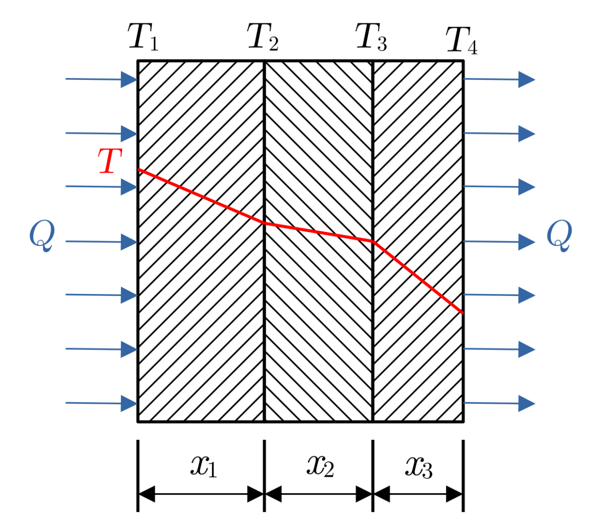
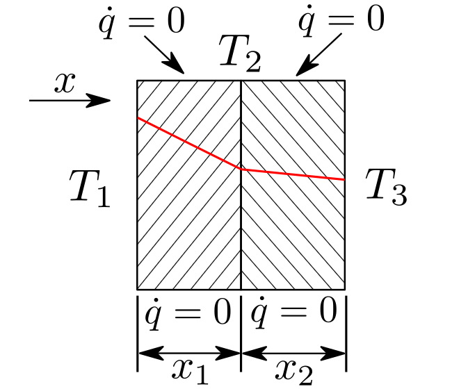
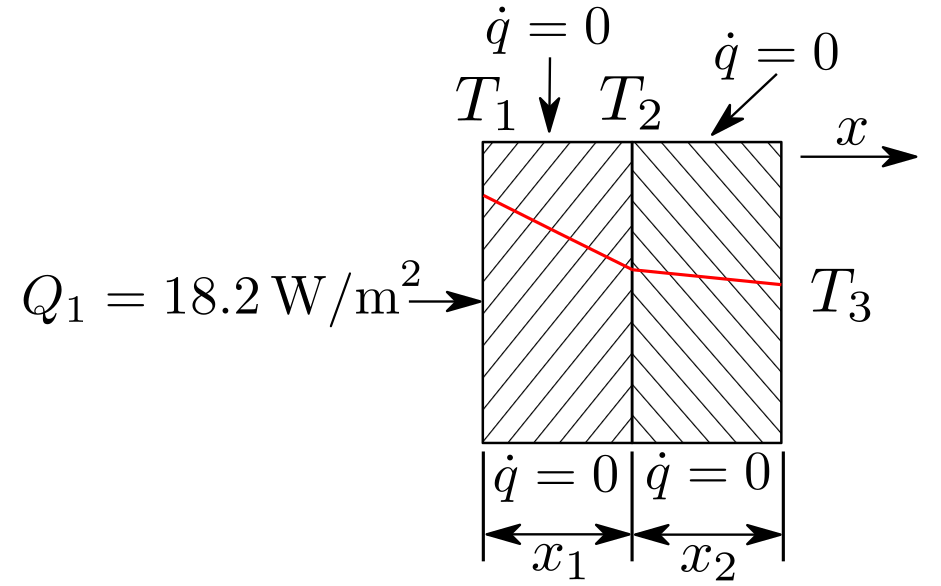
In this case, the uniform heat flux is: $$ Q = \frac{(T_1 – T_3)}{\left[ \frac{x_1}{k_1 A} + \frac{x_2}{k_2 A}\right]} \hspace{1.5cm}(5)$$

where:

  • \(k_1 = k_2 = 1\) W.m\(^{-1}\).K\(^{-1}\)
  • \(x_1 = x_2 = 0.5\) m
  • \(T_1 = 10\) °C
  • \(T_3 = 0\) °C

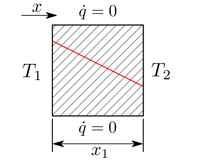
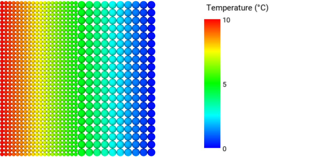
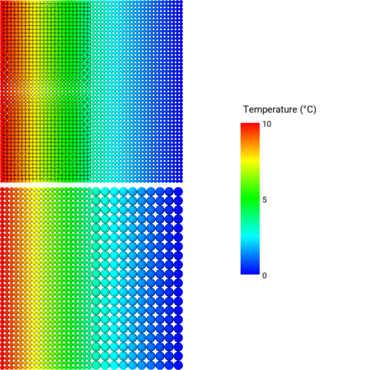
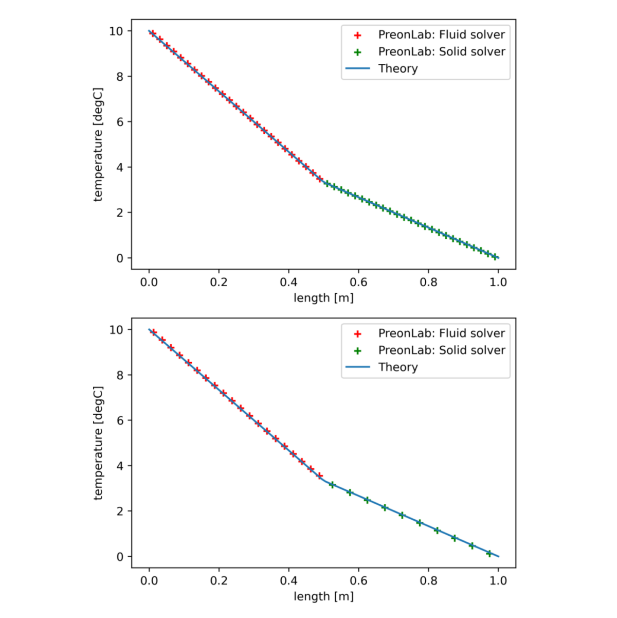
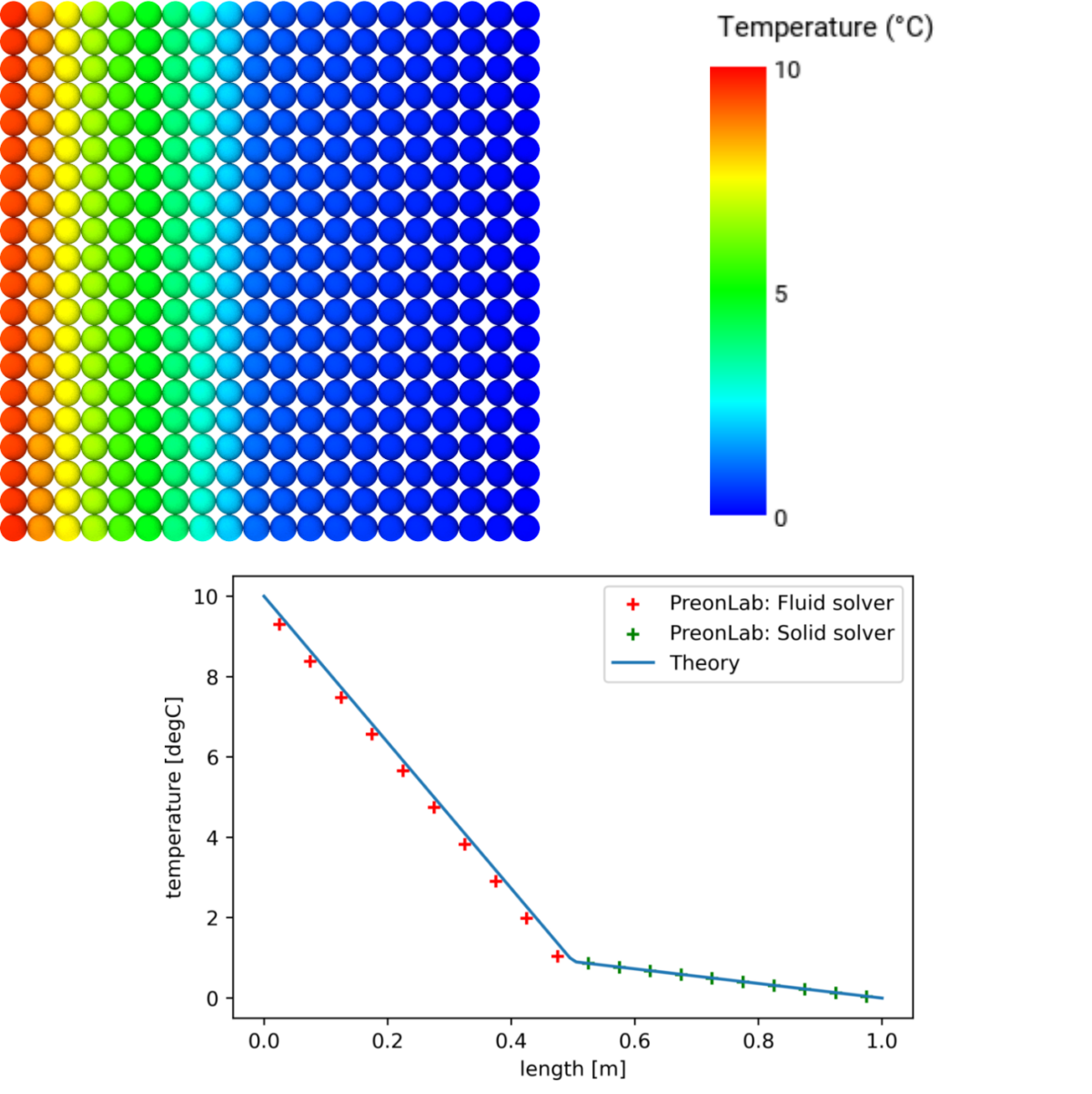
The temperature at the interface of the two solvers, \(T_2\), can now be computed using: $$ T_2 = T_1 – \frac{Q x_1}{k_1 A}\hspace{1.5cm}(6) $$ For this configuration the resulting heat flux and interface temperature are: \(Q = 10\) W/m\(^2\) and \(T_2 = 5\) °C. Since the conductivity is uniform throughout the wall Equation 1 can be used again to obtain the theoretical temperature distribution. In PreonLab the left layer contains a fluid solver and the right layer contains a solid solver. For a uniform spacing of \(20\) mm the results from PreonLab are:

  • \(Q_1 = 10.05\) W/m\(^2\) (\(0.5\) %)
  • \(Q_2 = 9.24\) W/m\(^2\) (\(-7.6\) %)
  • \(T_2 = 4.87\) °C (\(-2.6\) %)

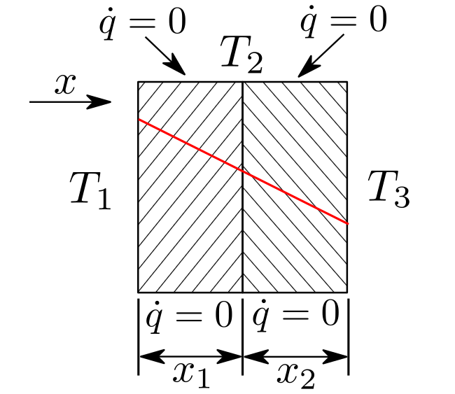
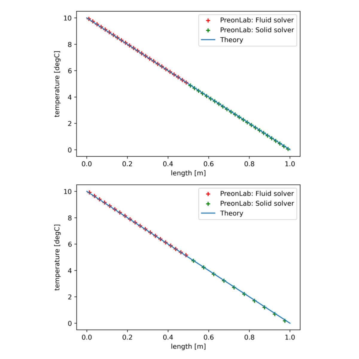
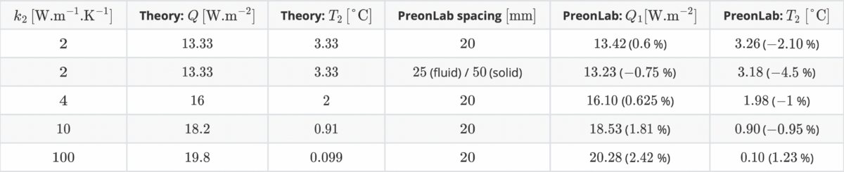
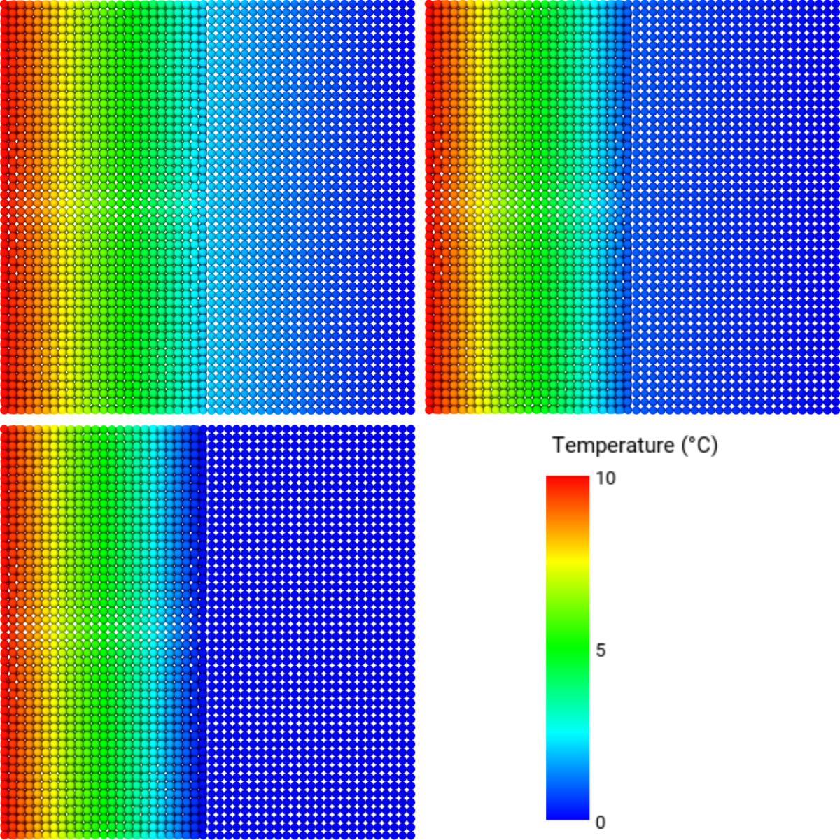
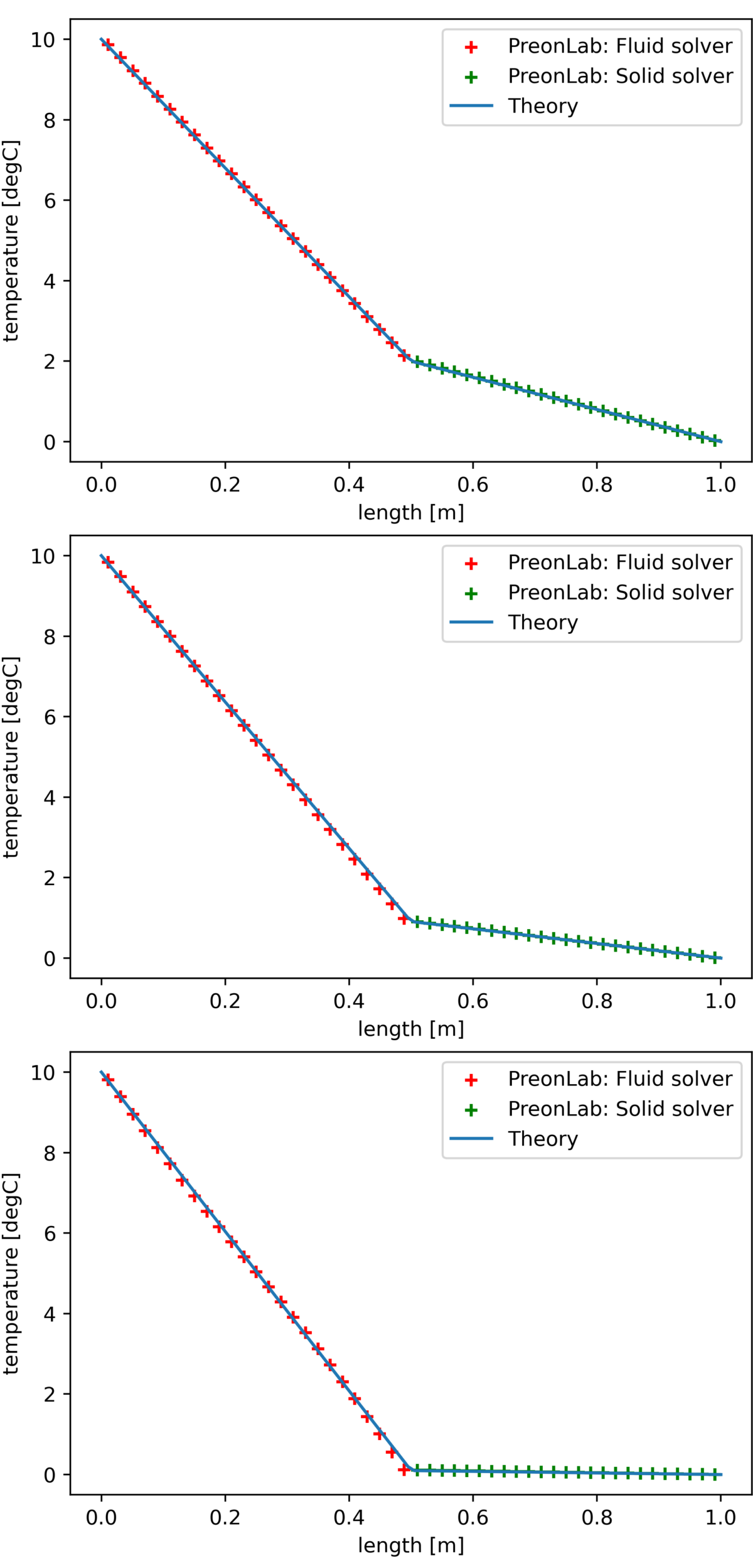
PreonLab also allows setting independent spacing for each solver. This feature is tested here with the following spacings:

  • Fluid spacing (left part) = \(25\) mm

  • Solid spacing (right part) = \(50\) mm

The temperature distribution for each configuration along the centerline of the wall is presented in Figures 5 and 6. The heat transfer between solvers behaves as expected.

Figure 5: Resulting temperature field for a heterogenous spacing configuration.

Figure 6: Temperature distribution of case 2 for uniform spacing (top) and heterogenous spacing (bottom).

Case 3 – 2 Layers 2 Materials

The next step in terms of complexity is to change the conductivity of one phase to alter the internal temperature distribution (see Figure 7).

Figure 7: Setup for case 3.

The parameters for this configuration are:

  • \(x_1 = x_2 = 0.5\) m
  • \(T_1 = 10\) °C
  • \(T_3 = 0\) °C
  • \(k_1 = 1\) W.m\(^{-1}\).K\(^{-1}\)

Equations 5 and 6 can also be used to obtain respectively the heat flux and the temperature between the solvers. The temperature distribution in each phase is:

$$ T\left(x\right)=\begin{cases}
0\leq x\leq x_{1} & \Rightarrow T_{1}-\frac{Q}{A}\frac{x}{k_{1}}\\
x_{1}\leq x\leq x_{2} & \Rightarrow T_{1}-\frac{Q}{A}\left(\frac{x_{1}}{k_{1}}+\frac{\left(x-x_1\right)}{k_{2}}\right)
\end{cases}\hspace{1.5cm}(7) $$
The various configurations and their results are summarized in Table 1.

Table 1: Summary of the various configurations together with their results.

In Figures 8 and 9, the comparison between uniform and heterogenous spacing is provided and shows good agreement with the theory. As expected the temperature gradient changes in each layer due to the change in conductivity. A higher conductivity leads to a lower temperature gradient. That behavior is confirmed in Figures 10 and 11 where the effect of increasing the conductivity of the second layer \(k_2\) can be observed. Each time, a good match with the theory is obtained.

Figure 8: Simulation result for \(k_2 = 2 \) W.m\(^{-1}\).K\(^{-1}\) with heterogenous spacing. Fine spacing for the fluid solver (top left) and coarse spacing for the solid solver (bottom left).

Figure 9: Temperature distribution for \(k_2 = 2 \) W.m\(^{-1}\).K\(^{-1}\) with uniform spacing (top) and heterogenous spacing (bottom).

Figure 10: Rendered result of the temperature distribution for \(k_2 = 4\) (top left),
\(10\) (top right), and \(100\) (bottom left) W.m\(^{-1}\).K\(^{-1}\).

Figure 11: Temperature distribution for \(k_2 = 4\) (top), \(10\) (center),

and \(100\) (bottom) W.m\(^{-1}\).K\(^{-1}\).

Case 4 – 1 Layer with Heat Flux Boundary Condition

The temperature boundary condition can now be changed to a heat flux boundary condition for verification (see Figure 12).

Figure 12: Setup for 1 layer with heat flux boundary condition.

We can use Equation 3 to get the temperature on the left wall: $$ T_1 = T_2 + \frac{Q}{k_1 A}x_1\hspace{1.5cm}(8) $$

where:

  • \(k_1 = 1\) W.m\(^{-1}\).K\(^{-1}\)
  • \(x_1 = 1\) m
  • \(T_2 = 0\) °C
  • \(Q = 10\) W/m\(^2\)

The theoretical temperature on the left side \(T_1\) is \(10\) °C. In PreonLab for a spacing of \(20\) mm, the measured temperature on the left side is \(9.91\) °C (\(-0.9\) %). Equation 4 can be used again to estimate the theoretical temperature distribution within the wall. The rendered result and the temperature distribution are shown in Figure 13.

Figure 13: Resulting temperature field (top) and temperature distribution along the centerline of the wall (bottom).

Case 5 – 2 Layers 2 Materials Heat Flux BC

Again a second layer with a different thermal conductivity like case 3 is added to the case with a heat flux boundary condition (see Figure 14).

Figure 14: Setup for Case 5.

Using Equation 5 we can get the temperature on the left wall: $$T_{1}=Q\left[\frac{x_{1}}{k_{1}A}+\frac{x_{2}}{k_{2}A}\right]+T_{3}\hspace{1.5cm}(9) $$

where:

  • \(k_1 = 1\) W.m\(^{-1}\).K\(^{-1}\)
  • \(k_2 = 10\) W.m\(^{-1}\).K\(^{-1}\)
  • \(x_1 = x_2 = 0.5\) m
  • \(T_3 = 0\) °C
  • \(Q_1 = 18.2\) W/m\(^2\)

The theoretical temperature on the left side \(T_1\) is \(10\) °C. In PreonLab for a spacing of \(20\) mm, the measured temperature on the left side is \(9.96\) °C (\(-0.4\) %). Equation 7 can be used again to estimate the theoretical temperature distribution inside the wall. The rendering of the result and the comparison of the temperature distribution between the simulation and analytical model are shown in Figure 15.

Figure 15: Resulting temperature field (top) and temperature distribution along the centerline of the wall (bottom).

Conclusion

PreonLab simulations have been validated against analytical solutions for a variety of configurations for the composite wall benchmark. Most notably the CHT implementation is producing reliable results. Heterogenous spacings have also been tested and validated. Finally, the main thermal boundary conditions (temperature and heat flux) showed good results.

Bibliography

[1] Lewis, R. W., Nithiarasu, P., and Seetharamu, K. N., Fundamentals of the finite element method for heat and fluid flow. 2004, John Wiley & Sons.

RELATED ARTICLES

LEARN MORE ABOUT PreonLab Updates

How to get started with
Preonlab CFD software?
Get in Touch