The next level
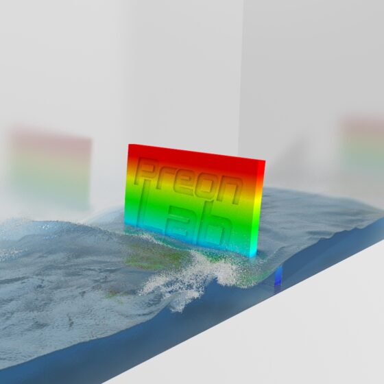
Adaptive Particle-based Simulation in PreonLab

March 09, 2021
Andreas Henne, Stefan Karch and Saba Golshaahi Sumesaraayi

Particle-based fluid simulation methods such as implicit SPH have many advantages over Eulerian grid-based methods. You can read all about it here.
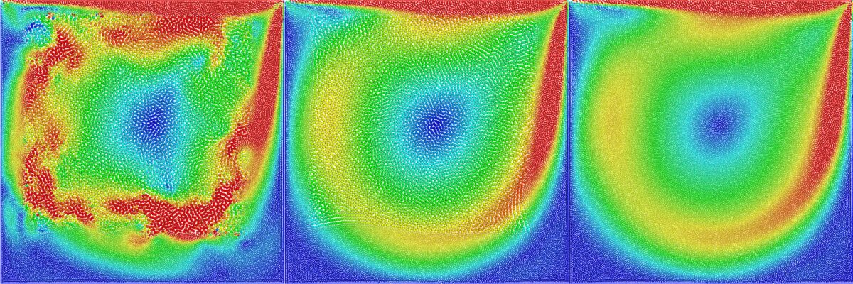
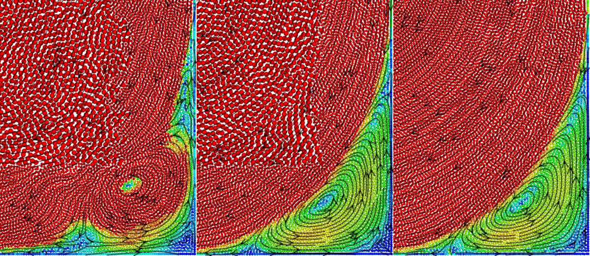
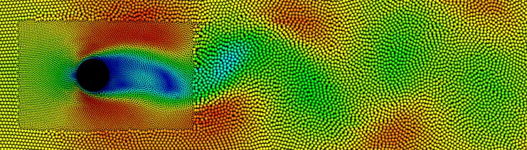
One advantage that Eulerian approaches still enjoy over most particle-based solvers is the ability to model fluid adaptively. By using finer cells in regions of interest and coarser cells in others, an adaptive mesh can reduce computational effort by several orders of magnitude. If multiple levels of detail are so clearly beneficial, why are they still relatively rare for most particle-based solvers?

Share:

Why particle-based adaptive simulations can be difficult

Figure 1: Velocity field of lid driven cavity simulation in PreonLab (with 1m/s lid speed, Re=1000, blue=0.0m/s, green=0.25 m/s, red=0.5 m/s). Left: Two particle levels (smaller particles near the walls) and no correction. Middle: Two levels and correction. Right: Uniform particle size. Without correction, the sudden changes in the particle distribution due to splitting or merging particles lead to unstable simulation results. For a closeup, see figure 2.

The idea

The basic idea for an adaptive particle-based solver is simple:

  • Allow for particles of different sizes in a simulation.
  • Split coarse particles if they get near regions of interest.
  • Merge fine particles if they leave regions of interest.

How difficult can this splitting and merging be? It all depends on the specific solver you are using. The Preon solver derives the density field directly from the distribution of particles. With this approach, a particle does not carry a property “density” over time, instead its density is computed from the distribution of nearby particles. This effectively prevents any compression over time due to the accumulation of numerical errors. However, if you want to build an adaptive solver, this blessing becomes a curse. Splitting and merging inevitably changes the distribution of particles. Therefore, it also changes the density field which in turn can lead to artificial pressure forces.
The goal of an adaptive solver is to accelerate simulations. But it is useless if the simulation results are wrong – smaller particles do not automatically give you a better result! The image on the left in figure 1 shows this problem in a lid-driven cavity setup (read more about it here). Particles near the center are coarsened while particles near the boundary are refined. The artificial pressure forces due to splitting and merging violently disturb the velocity field and no stable state is reached.

Preserving the density field

Figure 2: Closeup of bottom right corner for two particle levels and no correction (left), two levels and correction (middle) and uniform particle size (right). The coloring (blue=0.0m/s, green = 0.01m/s and red=0.04m/s) is chosen to emphasize the vortices in the corners. Additionally, streamlines are plotted to show velocity directions. The adaptive simulation with correction matches the results of the uniform simulation well.

So how do we deal with these sudden changes in the particle distribution? Moving to a differential density update (as some other SPH solvers do) could help, but this would also create other challenges (most notably the prevention of compression over time). We also wanted to match our existing solver as close as possible to verify the results. We opted for a dedicated solver step to optimize the particle distribution so that it approximately matches the density field as it was before the splitting or merging. This works well but also adds a significant computational effort. For PreonLab 5.0, we also adapted our implicit pressure solver so that this correction can be split into smaller changes across multiple simulation steps. This relaxes the burden on the correction step and improves overall performance if splitting and merging occurs often.

The lid-driven cavity is a perfect benchmark to verify this correction, because any artificial pressure forces will quickly distort the slow vortices that are expected to form in the corners. Figure 1 (middle) shows how the simulation with two particle levels and correction enabled reproduces the velocity field of the simulation with one particle level (right) well. Figure 2 shows a closeup of the bottom right corner with adjusted coloring to see the slow vortex that is expected to form there. With the correction enabled, we can almost perfectly reproduce the simulation results of the uniform simulation. This also indicates that the correction does not introduce artificial viscosity, which would smooth the velocity field.

But what about computation times?

Knowing that our adaptive solver matches the high-resolution uniform simulation for the lid driven cavity allows us to have confidence in the method. However at the end of the day, we are interested in computation times.

Read this article to learn how PreonLab 5.0 overcomes the limitations of PreonLab 4.x to deliver unprecedented speedups.

RELATED ARTICLES

LEARN MORE ABOUT PreonLab Updates

How to get started with
Preonlab CFD software?
Get in Touch